TestPlayer 2.0 – User Manual

Abstract

TestPlayer 2.0 is an advanced, web-based platform for Model-Based Testing (MBT) [1] that automates the creation of test suites from state transition models. Users can utilize an integrated development environment to edit DOT graphs [2] and define stochastic user profiles via Markov Chain Usage Models (MCUM). The system features an MBT Wizard for configuring test algorithms, such as node and edge coverage, and an SUT Adapter Manager to link abstract models with real-world browser interactions [4]. A hierarchical Project Workspace organizes the generated artifacts, while interactive dashboards provide analytical metrics like steady-state probabilities. Extensive visualization tools [3] allow for the step-by-step inspection of test cases and comparative performance analysis of test runs. Ultimately, the platform streamlines the entire testing lifecycle—from automated model generation through UI crawling to the detailed reporting of execution results.

1. Login and Authentication

Access to TestPlayer 2.0 is protected by a secure authentication system.

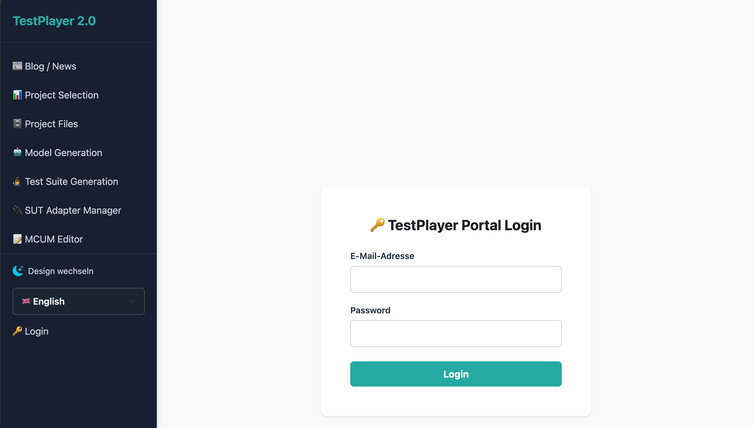
Figure 1 The central login screen of the TestPlayer portal.

After successfully entering the email address and password, the user is redirected to their personal workspace.

2. Dashboard and Model Management

The dashboard is the central entry point and the personal control center after logging in. All available test models (projects) of the logged-in user are listed here.

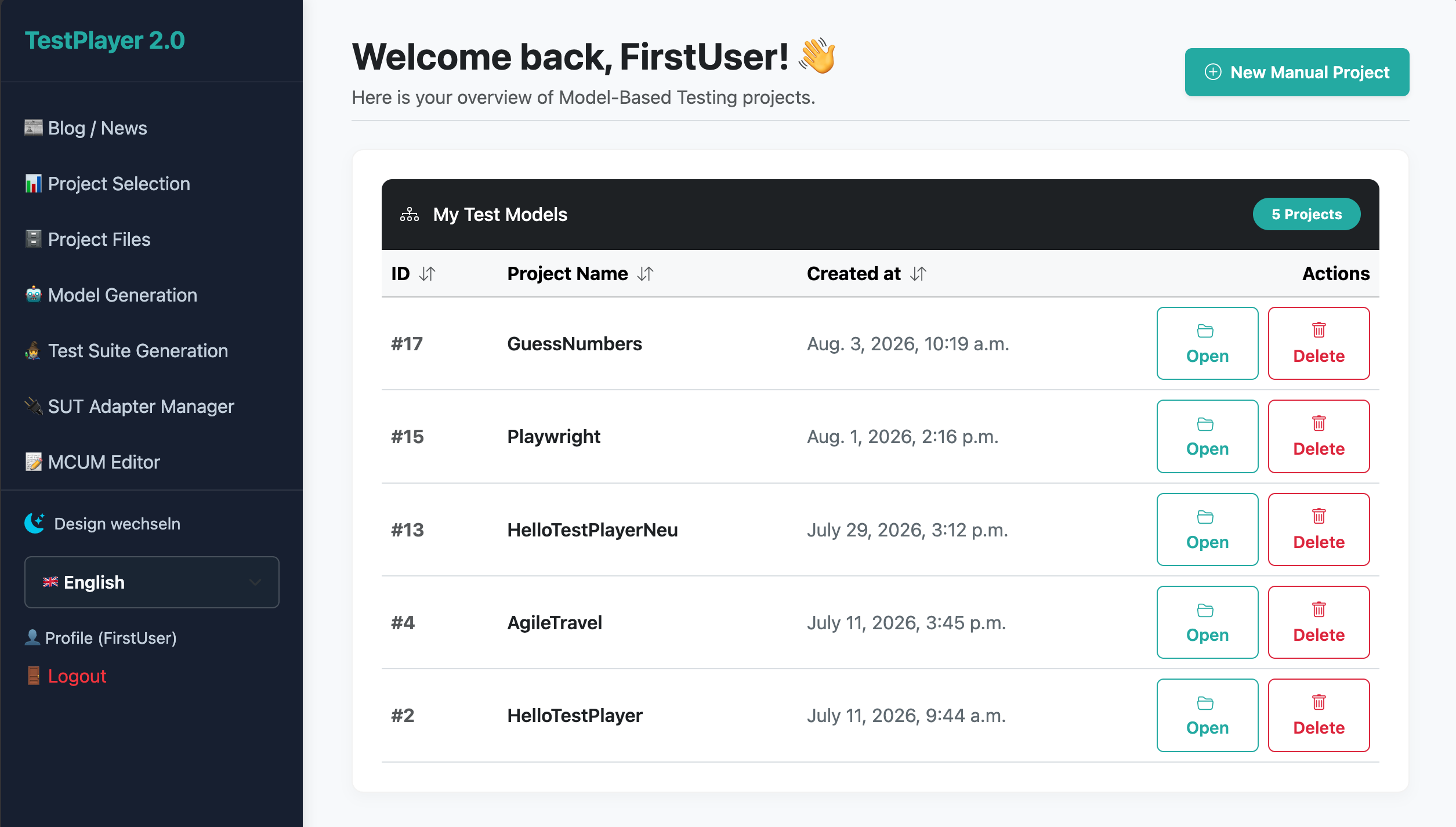
Figure 2 The personalized dashboard overview of the user’s test models.

• Project Selection: Clicking on “Open” for a project leads directly to the project files, where all generated artifacts are managed.

• New Project: Fresh DOT models can be imported into the system and prepared for test generation via the “+ New Project” button.

3. Blog / News & Updates

To stay informed about new features, releases, and announcements regarding Model-Based Testing, TestPlayer 2.0 features an integrated blog section.

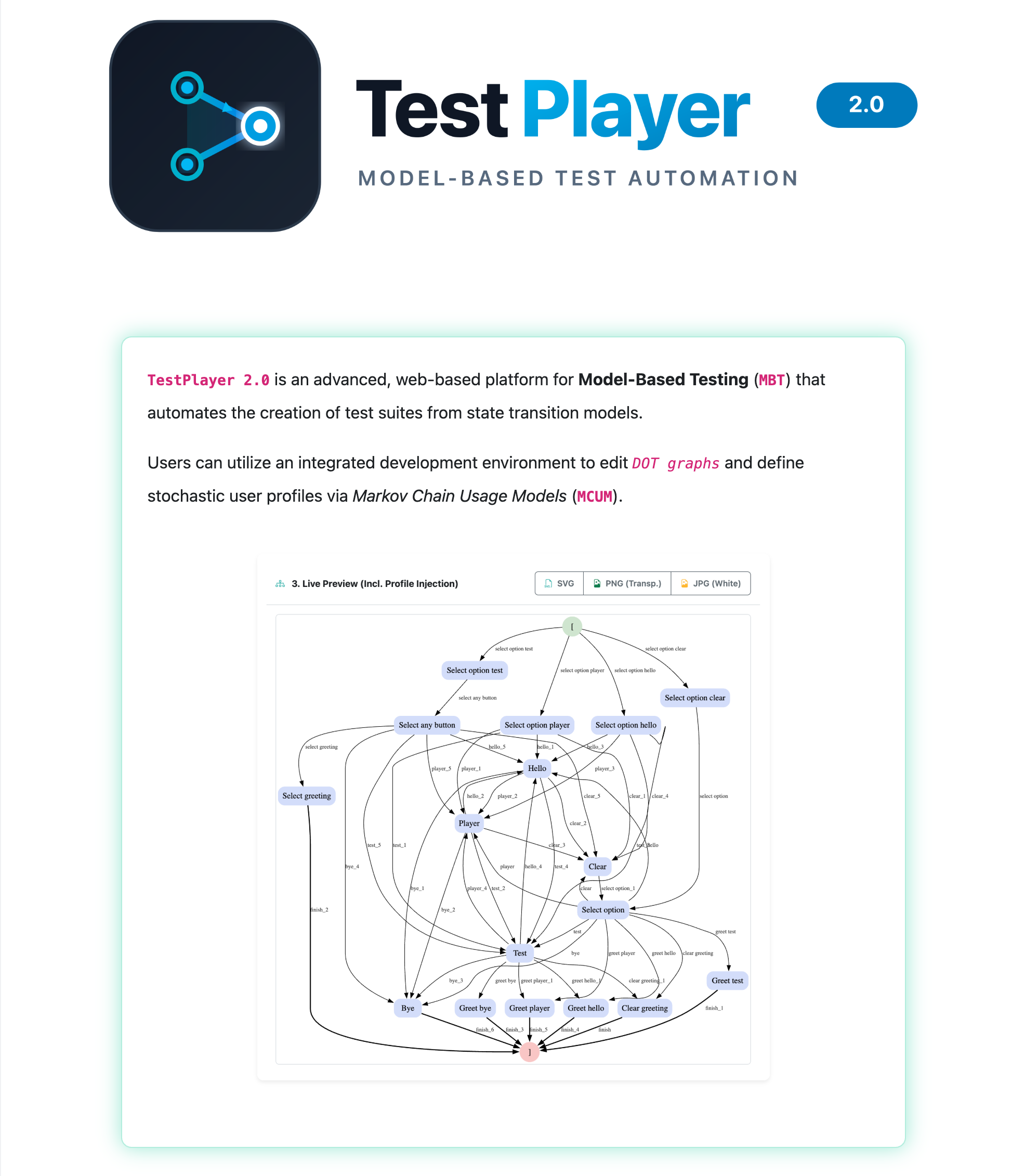
Figure 3 The news section for current release notes and announcements.

4. DOT Editor & MCUM IDE

The integrated development environment (IDE) of TestPlayer 2.0 allows direct editing of the graphs and probabilities directly in the browser, divided into base model editing and profile management.

4.1 Edit Base Model

In the upper area of the IDE, the DOT code of the base model can be edited [2].

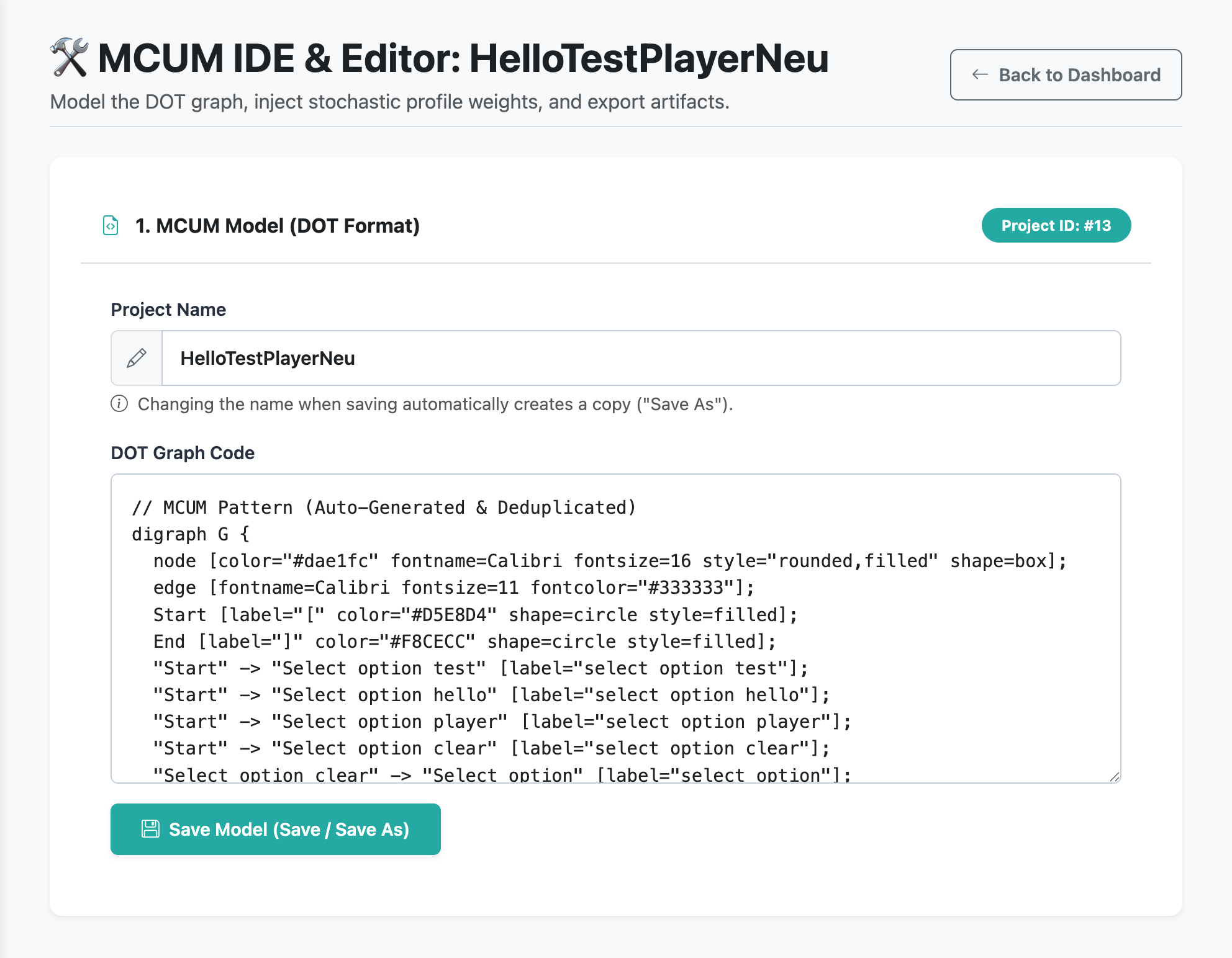
Figure 4 Code editor for the underlying DOT model.

Every change to the code can be visually verified immediately. The live preview renders the base model and displays the topological structure (“Ground Truth”).

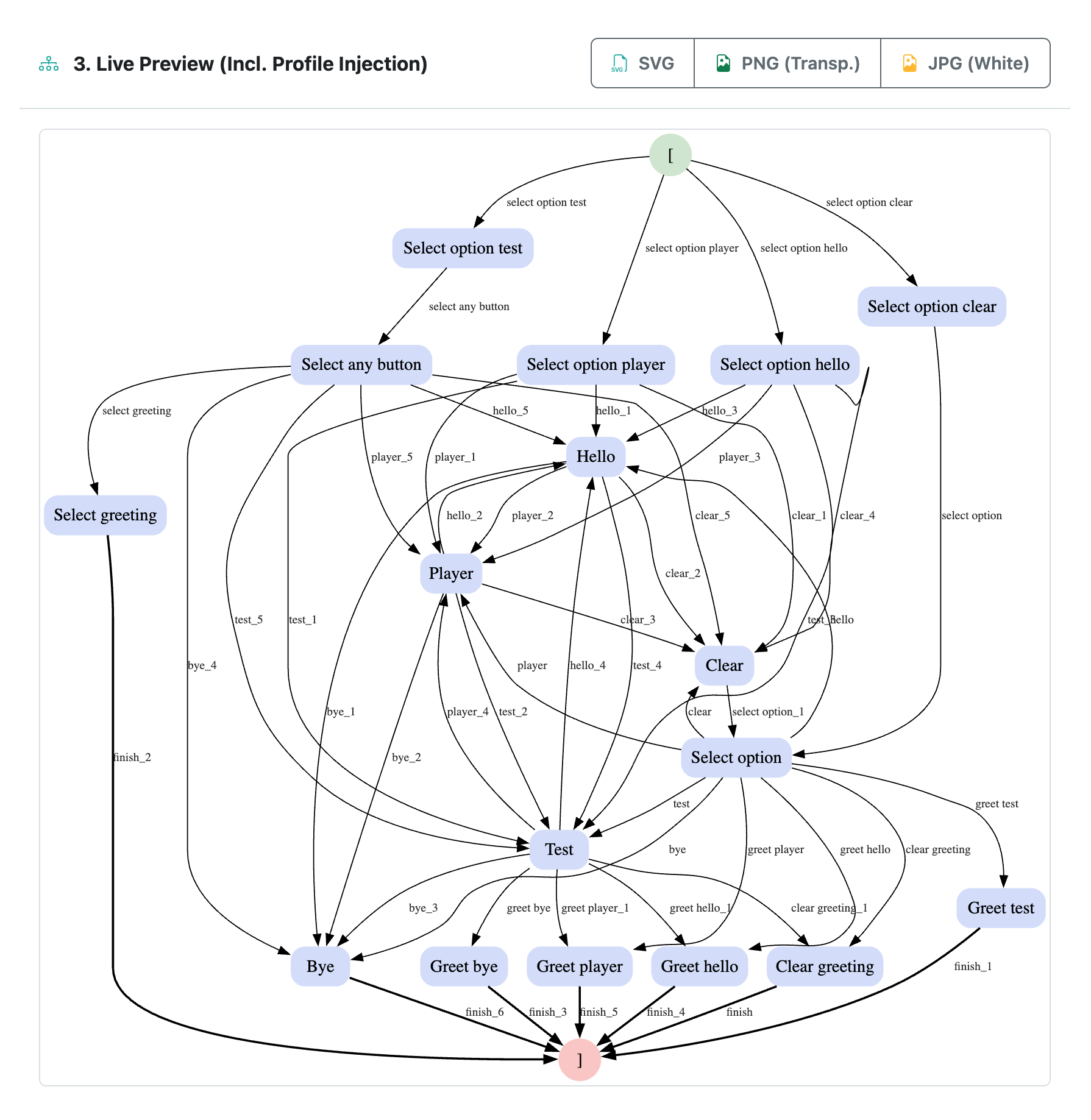
Figure 5 Rendered live preview of the base model.

4.2 Profile Management & Live Injection

In the lower area of the IDE, user-specific profiles (e.g., HappyPath) can be created and managed in JSON format. These profiles overwrite abstract variables in the DOT code with concrete transition probabilities.

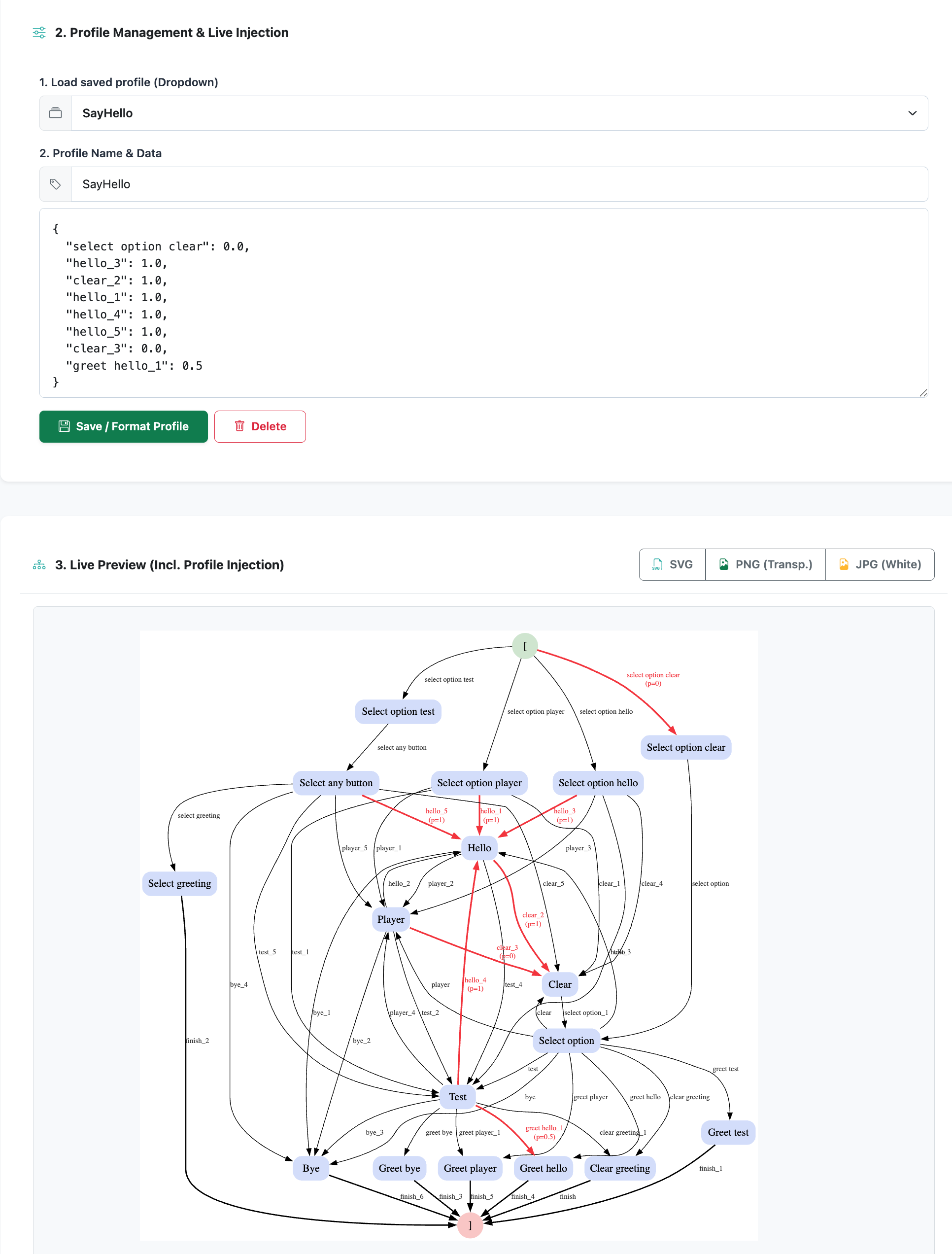
Figure 6 Management and editing of stochastic user profiles.

As soon as a profile is selected, the live preview projects the stochastic weights directly onto the graph. The edges are colored and highlighted according to the injected probabilities.

Note

Assignments of p=0 in a profile are strictly respected by the algorithm, so these edges are ignored during generation. Inaccessible parts of the graph are automatically isolated by the stochastic analysis.

5. The MBT Wizard (Parameter Configuration)

The MBT Wizard controls the Smart Testing Engine. In the first step, the desired model is selected from the personal library.

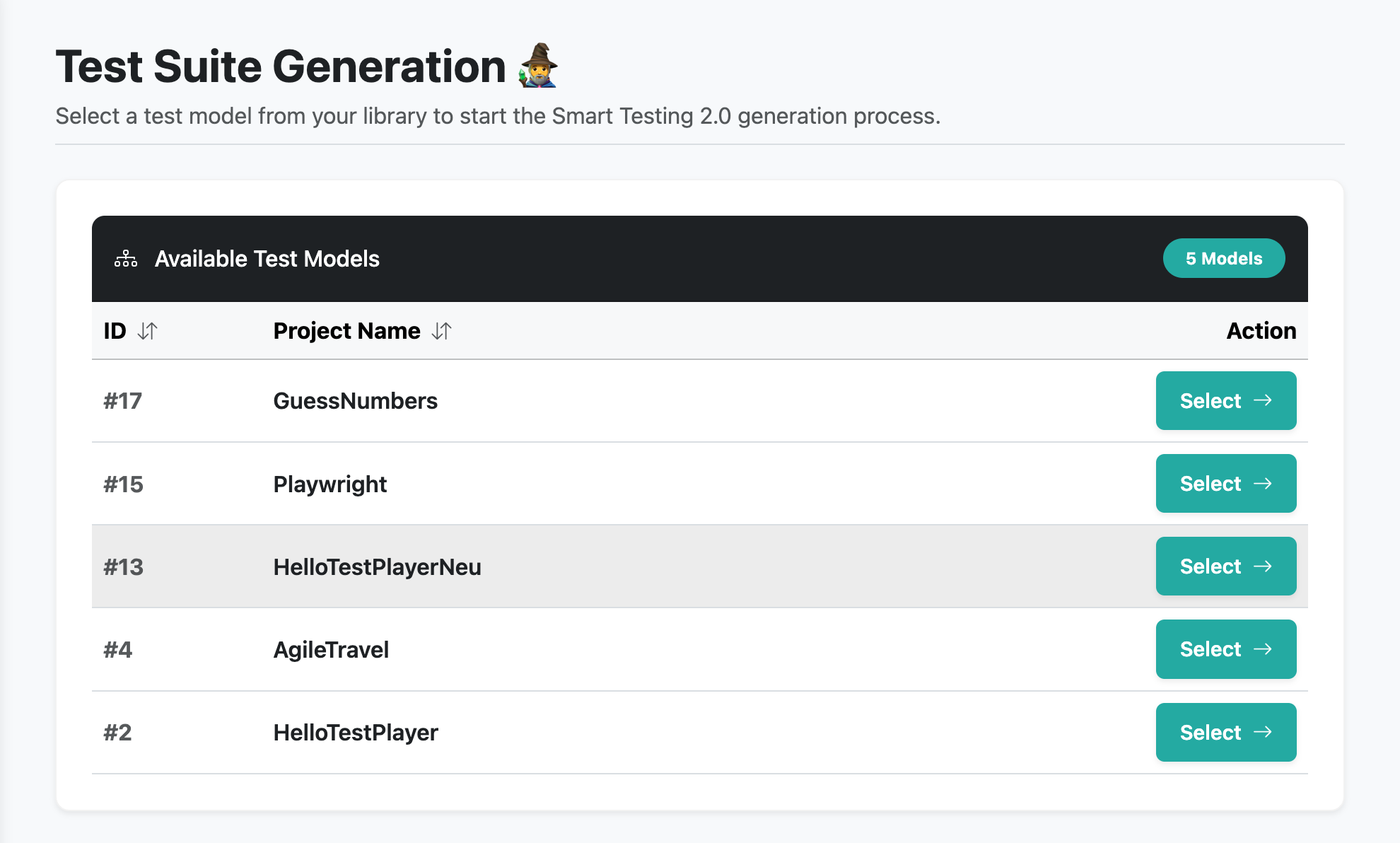
Figure 7 Start screen of the MBT Wizard for selecting the test model.

Subsequently, the parameters for generating the test suite are defined. The user interface automatically remembers the last used settings per project.

5.1 Test Algorithms

• Random Walk: Generates random paths through the model until the target state is reached or the maximum number of steps is attained.

• Node Coverage: Guarantees that every reachable node is traversed at least once. Redundant paths are eliminated by a greedy algorithm.

• Edge Coverage: Guarantees that every reachable edge is covered.

• Markov Chain Variants: Combines the above algorithms with the statistical probabilities from the profiles of the MCUM IDE.

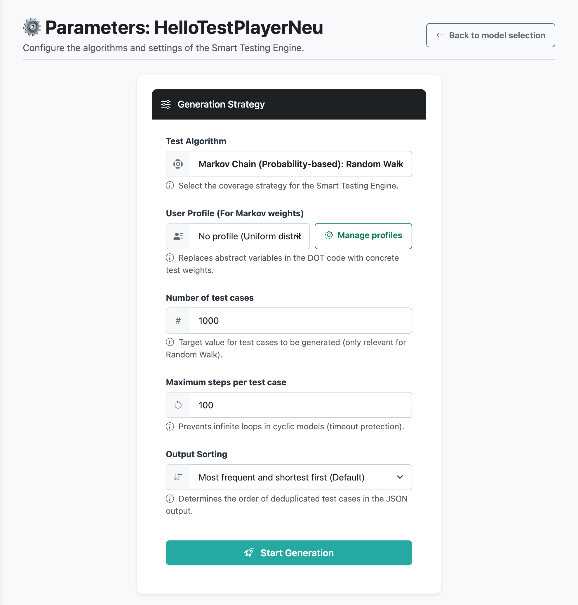
Figure 8 Algorithms for test case generation.

6. SUT Adapter Manager (Web UI)

A System Under Test (SUT) adapter forms the link between the abstract states and edges of the test model (e.g., e1, s2) and the concrete interactions of the test execution (Playwright Automation Engine [4]). A fully integrated web interface is available via the menu button 🔌 SUT-Adapter Manager, with which SUT adapters can be created, configured, and maintained.

6.1 Adapter Overview & Management

The main view of the manager provides a tabular list of all adapters existing in the system:

• Search and filter function: Enables quick location of adapters by name or target URL.

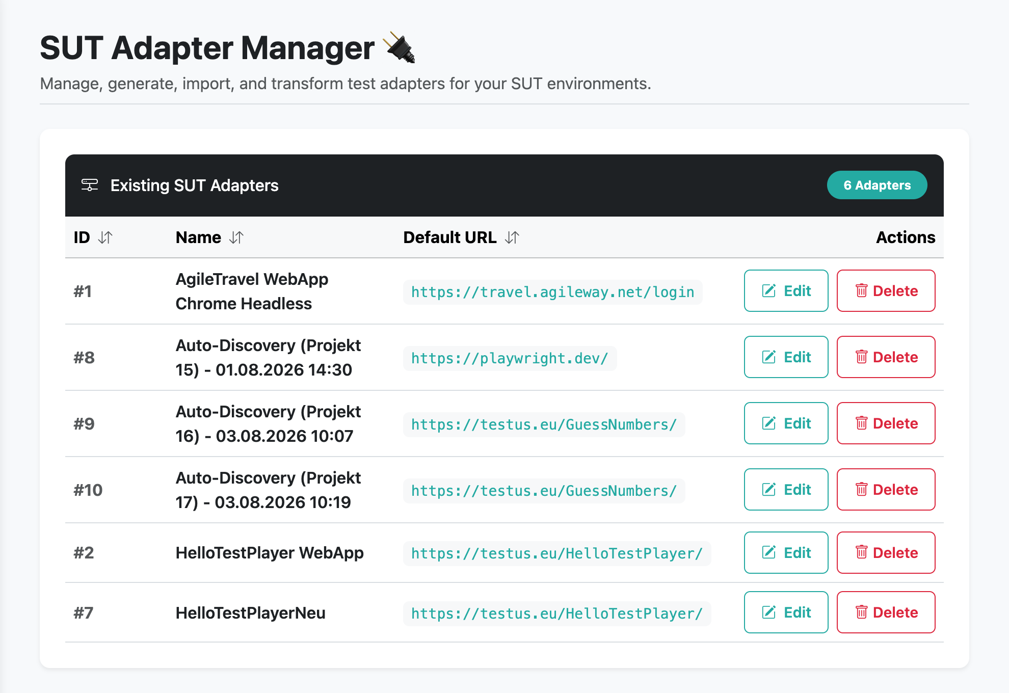
Figure 9 Overview and quick access to all configured SUT adapters.

• Creating new adapters: A new adapter container can be created directly in the user interface via the “+ New Adapter” button.

• Actions: Buttons are available for each adapter to directly open the detailed configuration as well as to securely delete obsolete instances.

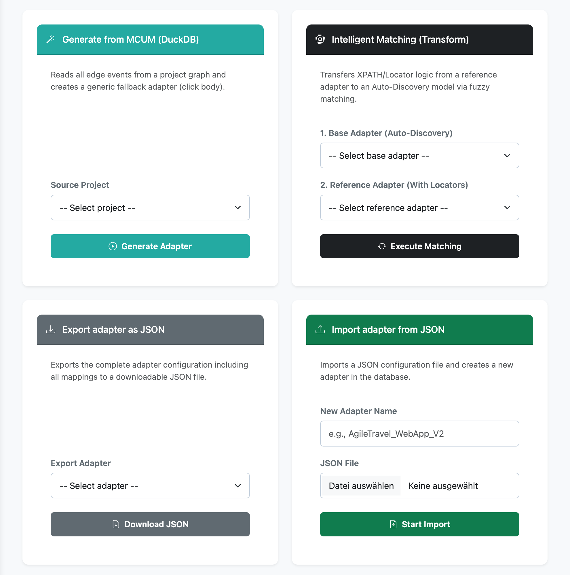
Figure 10 Creating new SUT adapters and further actions.

6.2 Master Data & Authentication

The detailed view of an SUT adapter is divided into a two-part working environment: On the left side is the form for maintaining the basic connection parameters.

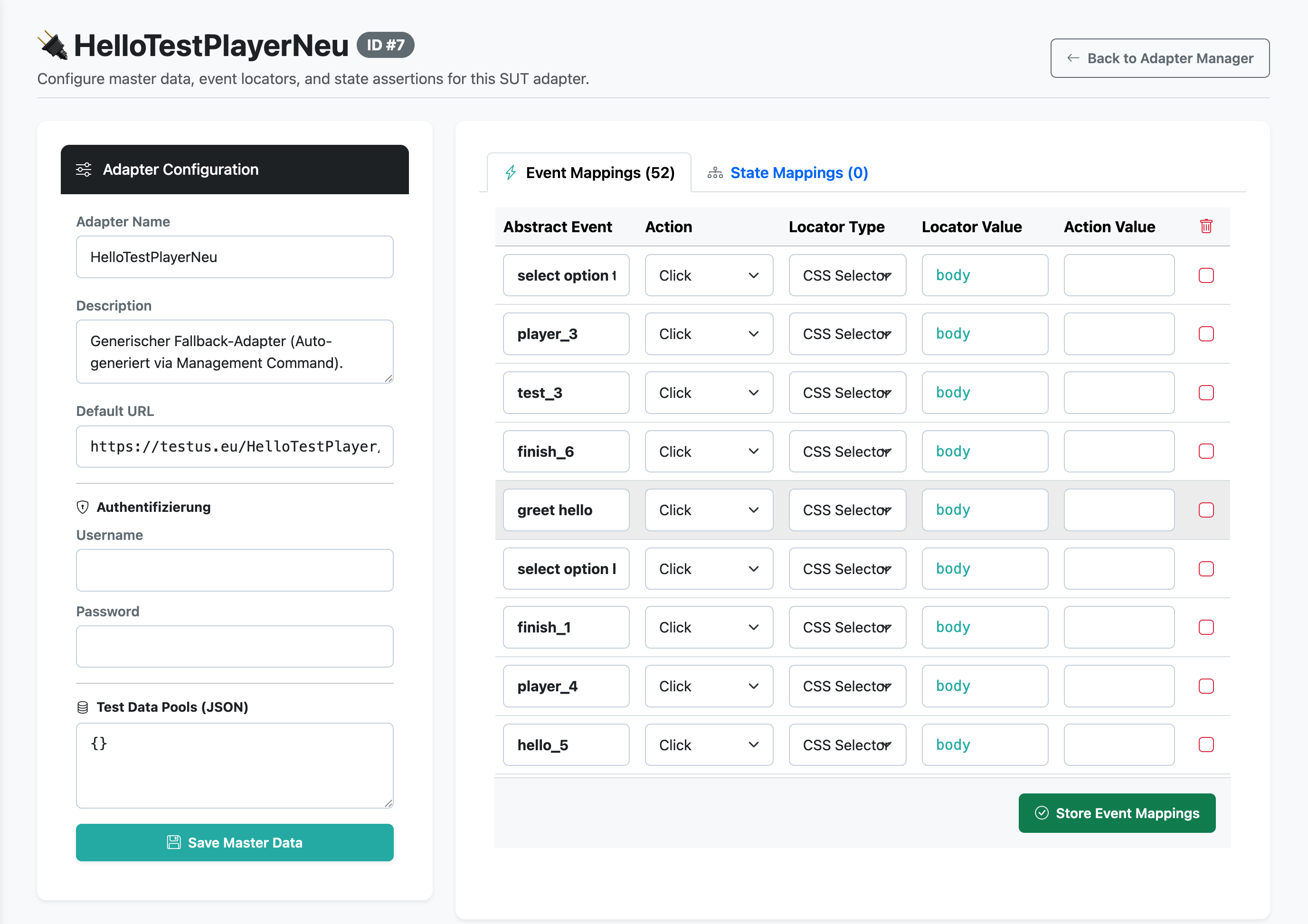
Figure 11 Master data panel for maintaining URLs, login data, and JSON test data.

1. Adapter Name & Description: Unique designation and free-text description for the test team.

2. Default URL (SUT Target): The base URL of the web system to be tested (e.g., https://localhost:8000).

3. Authentication (LOGIN_MACRO): Access data (Username and Password) that are automatically injected when a test step executes the Login Macro Flow action.

4. Test Data Pools (JSON): Key-value store in JSON format for providing dynamic input data. Variables in the form of {{variable}} within event mappings resolve values from this pool automatically at runtime.

6.3 Event Mappings Editor (Locators & Actions)

The interactive tab Event Mappings is located in the right-hand area. Here, it is defined which UI action is to be executed on the website when an abstract model event (e.g., player_4) is triggered.

Each event mapping includes the following parameters:

• Abstract Event: Name of the edge in the DOT model (e.g., player_4).

• Action (Choice): Predefined selection list of the interaction type:

• Click: Mouse click on an element.

• Text Input: Entering text into an input field.

• Submit Form: Submitting a form.

• Assert Element Visible: Checking visibility.

• Sleep / Wait: Defined waiting for UI reactions.

• Select Dropdown: Selecting an option from an HTML select box.

• Login Macro Flow: Executing the automated login process.

• Locator Type (Choice): Type of element finder:

• CSS Selector, ID, XPath, Name, Class Name, Link Text, Tag Name, None / Macro.

• Locator Value: The concrete search expression in the DOM (e.g., #btn-submit or //button[@id='login']).

• Action Value: Optional additional data for the action (e.g., the text to be entered or the variable {{username}}).

Note

In-Place Editing, Deleting & Adding: Changes in the table can be made directly. An assignment is deleted via the trash can icon at the end of the row. Another event mapping can be added to the table immediately via the highlighted green row at the end of the table (➕ New Event). Clicking on “Save Event Mappings” saves all adjustments collectively.

6.4 State Mappings Editor (Assertions & Indicators)

The second tab, State Mappings, regulates the test oracle: It defines how the TestPlayer verifies whether the SUT has successfully reached a certain model state (e.g., s5) after executing an event.

• Abstract State: Name of the state in the DOT model (e.g., s5).

• Indicator Type (Choice): Verification method for the state:

• CSS Selector (Visible): Checks whether a specific UI element is visible in the DOM.

• URL (Regex / Contains): Checks whether the current browser URL contains a pattern (e.g., /dashboard).

• Visible Text in DOM: Verifies the presence of a specific text section on the page.

• Indicator Value: The concrete value or search expression for the indicator (e.g., .logged-in-banner).

7. Project Files (Workspace)

The file view is strictly hierarchically structured (Profile \(\rightarrow\) Suite \(\rightarrow\) Artifacts) in order to maintain an overview even with hundreds of generated files.

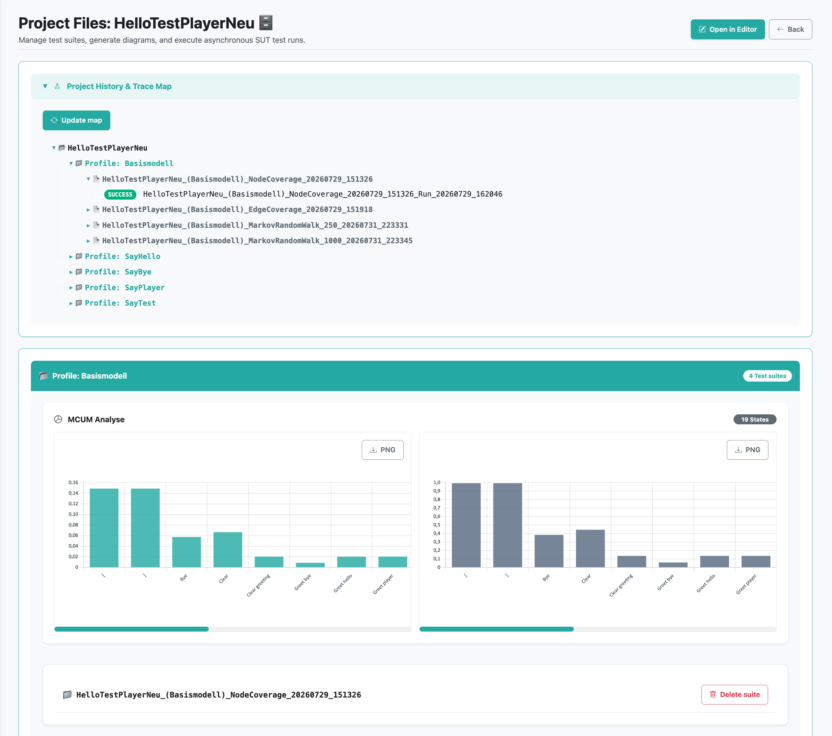
Figure 12 Overview of project files with profile folders.

Note

Dynamic visibility of profiles: The view of the project files is a dynamic file browser. The green profile folders are exclusively generated from the file names of the actually existing test suites. A newly created profile in the MCUM IDE (e.g., HappyPath) only appears here after at least one test suite has been generated for this profile via the MBT Wizard.

7.1 Folder Hierarchy

1. Profile Level: Green folders (e.g., Profile: Base model) that encapsulate all associated test suites.

2. Suite Level: The specific run. The complete test suite including all generated diagrams can be completely removed from the database here via the “🗑️ Delete suite” button.

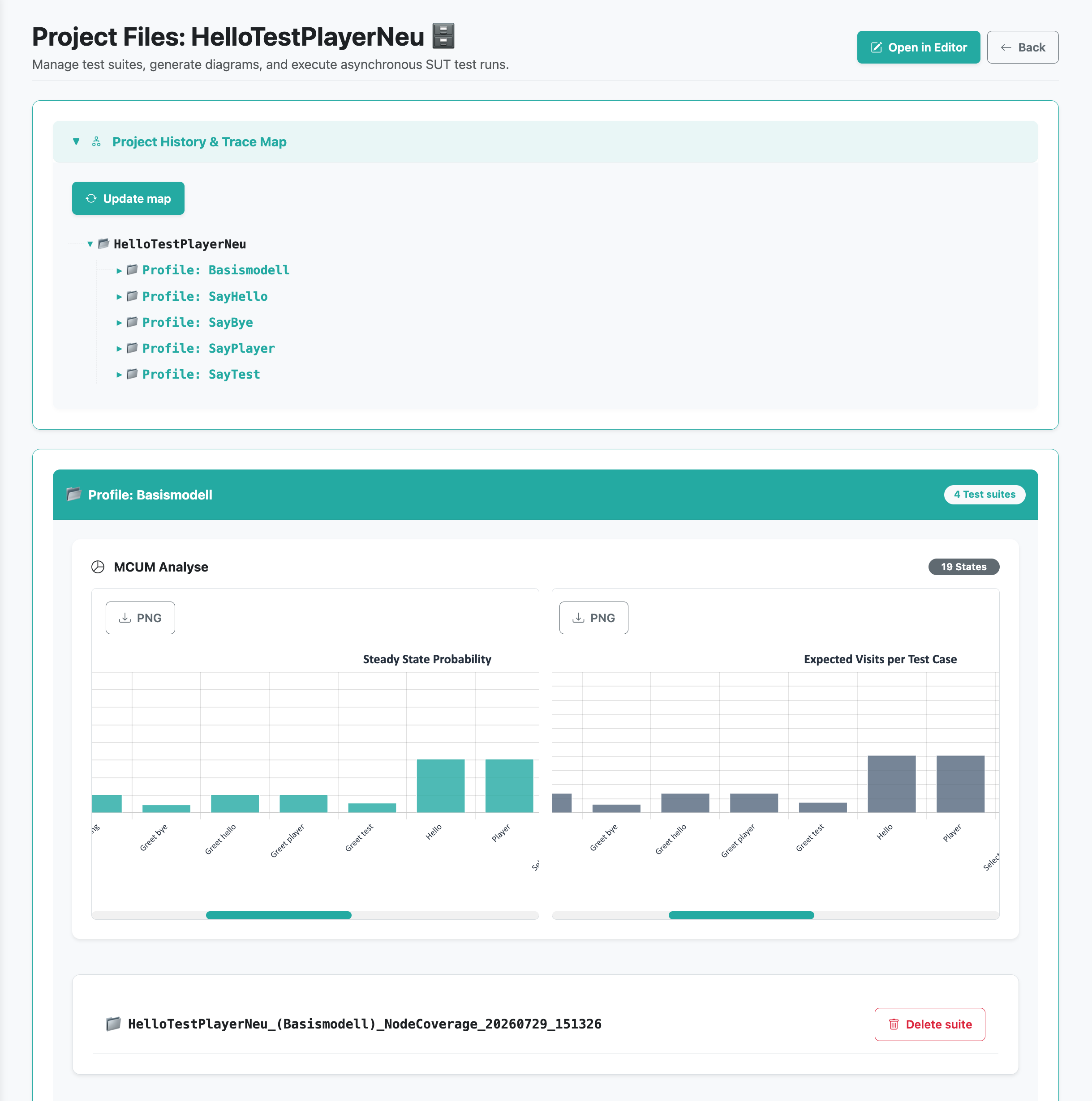
Figure 13 Profile/Testsuite-Level: Encapsulation of all associated test suites.

3. Artifact Level: Divided into expandable workflow phases 1. Test suite & Execution, 2. Diagrams & Artifacts, 3. Test runs (Reports & DuckDB Live-Traces) and 4. Visualization of the test runs.

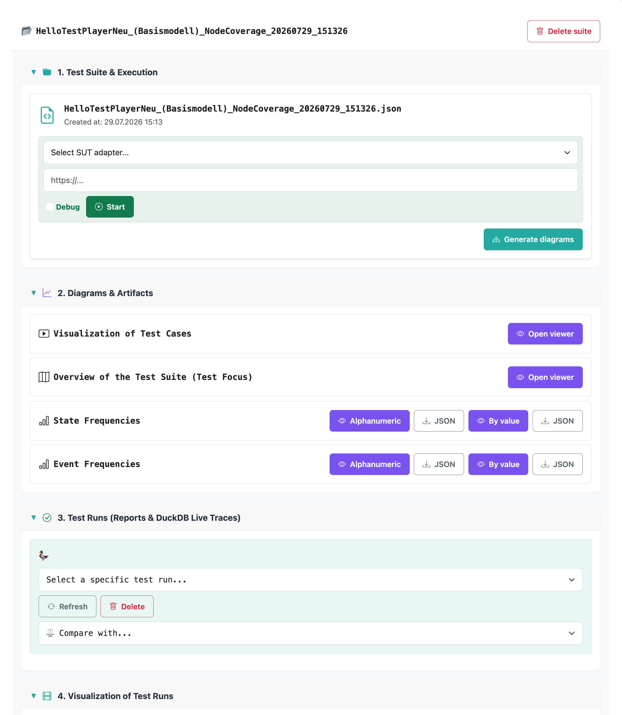
Figure 14 Artifact Level: Divided into expandable workflow phases.

7.2 MCUM Analysis Dashboard (Steady-State & Visits)

As soon as a profile folder is expanded, the Smart Testing Engine calculates the analytical metrics of the underlying Markov model on-the-fly via matrix operations (Fundamental Matrix \(N\)) [1]. The results are presented as:

• Steady State Probability: Shows the relative, long-term residence probability (\(\pi\)) for each state.

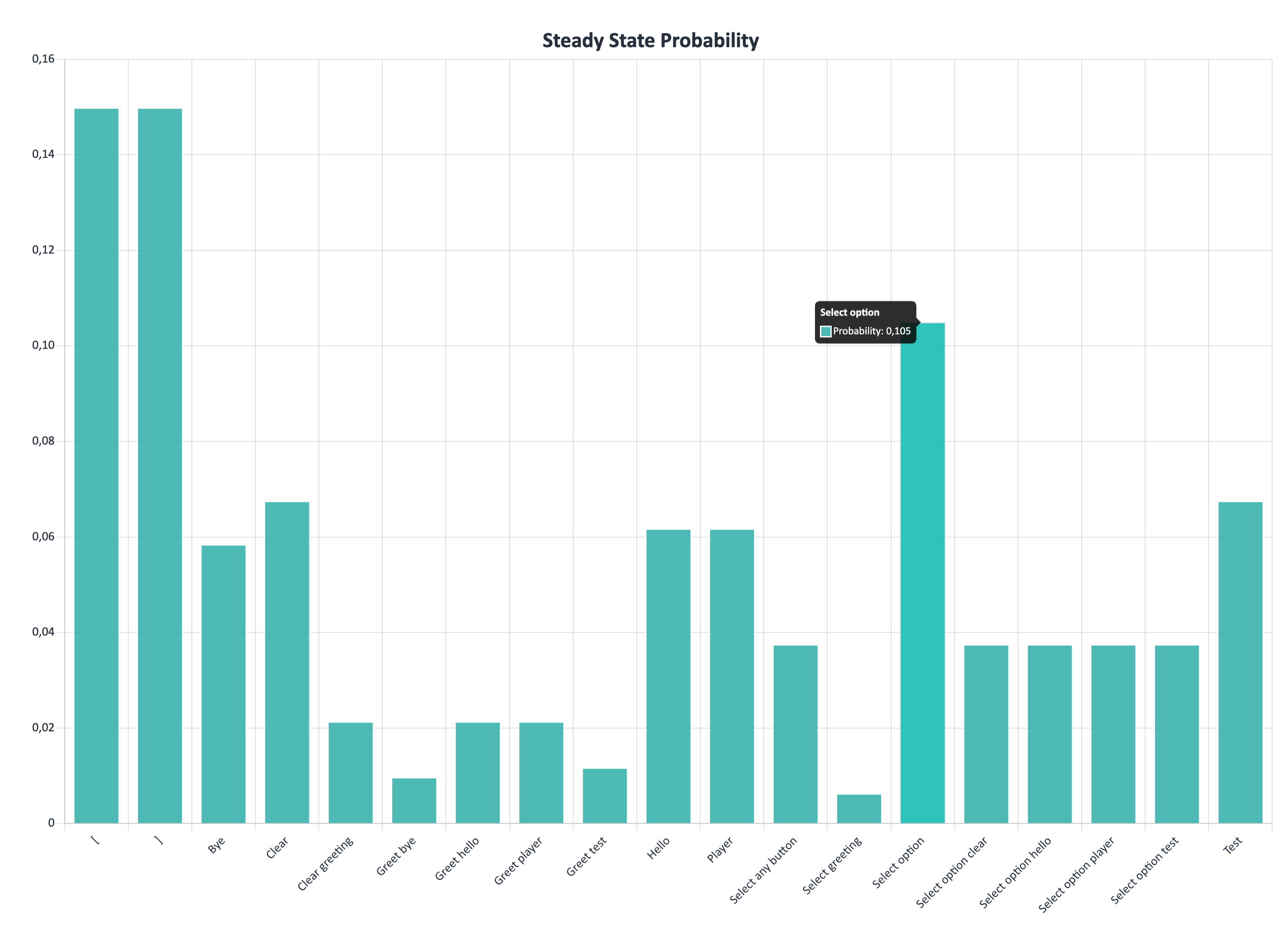
Figure 15 Steady State Probability: Relative residence probability (\(\pi\)) for each state.

• Expected Visits per Test Case: Shows the number of average visits (\(V\)) of a node per test run.

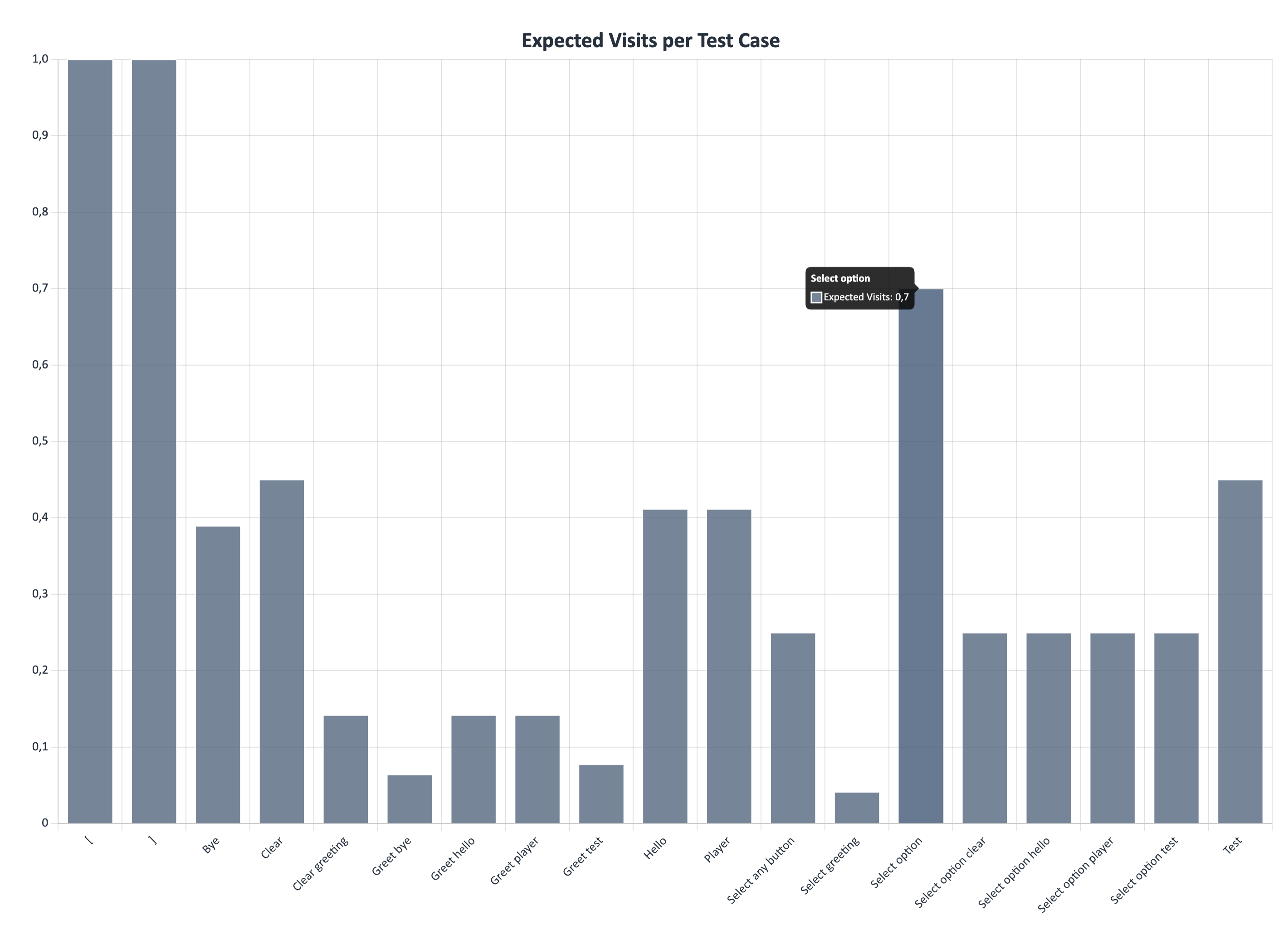
Figure 16 Expected Visits per Test Case: Number of average visits (\(V\)) of a node per test run.

Note

Why do both diagrams look identical? The fact that the bars have exactly the same relative height is a mathematical law of absorbing Markov chains [1]. The stationary probability of a node (\(\pi_i\)) is strictly proportional to its expected visits (\(V_i\)) divided by the average total length of a test case. The X-axis shows the states sorted alphanumerically.

7.3 Project Documentation & Timeline

At the bottom of a project’s files is the chronological project documentation. This vertical timeline serves as an audit log and seamlessly combines automatic system events with manual user annotations. To facilitate navigation even with long project histories, the timeline is collapsed by default and can be reversed at any time via a dedicated sort icon at the top (chronological / reverse chronological).

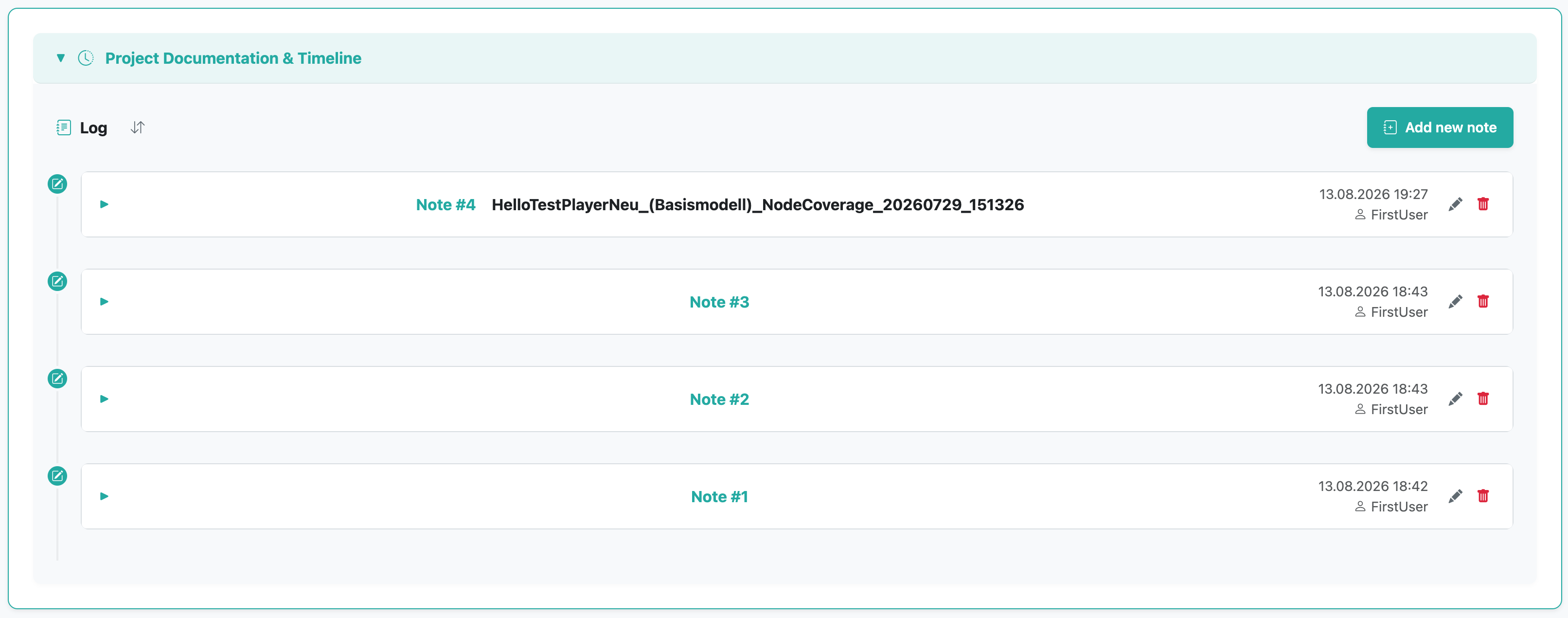
Figure 17 The project documentation aggregates test runs and collapsible manual notes in a sortable timeline.

Automatic System Events: As soon as an asynchronous test run is started, successfully completed, or aborted with an error, the system automatically generates an entry in the timeline. This allows the history of test executions to be traced visually and seamlessly.

Manual Notes & Markdown Editor: Via the “Add new note” button, domain testers can document their own observations, error analyses, or intermediate statuses. Manual notes are clearly displayed as expandable tabs (accordions), which are closed in their default state and only show their sequential number and assigned title.

• Title & Numbering: Each note is automatically assigned a sequential identification number by the system (e.g., “Note #4”) and can be given an optional, individual title for better discoverability.

• Markdown & Mermaid: The integrated editor supports full Markdown as well as Mermaid.js for quick sketching of diagrams.

• Live Preview: While typing, a live preview immediately displays the final, rendered result.

• Metadata Injection: New notes are automatically populated with a dynamic template that captures the date, time, and the tester’s current location (e.g., Waldaschaff).

• Multiple File Upload: Any number of screenshots and images (multiple selection) can be attached in a single step via the upload field. These can be flexibly arranged within the text using placeholders and are dynamically embedded into the final Markdown rendering.

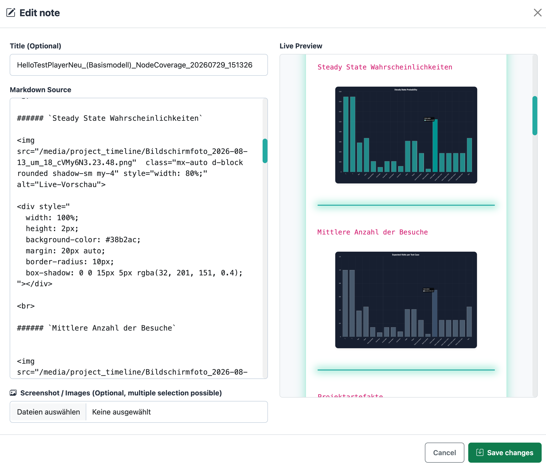
Figure 18 The editor offers live rendering for Markdown, customizable titles, and multiple image uploads including a metadata template.

Editing and Deleting Entries: Manual notes can be adjusted retrospectively at any time. Clicking the pencil icon (directly in the tab header) reopens the existing note in the editor to refine texts or the title and to upload additional images. Outdated entries can be irretrievably removed from the history using the trash can icon.

8. Visualization and Diagram Viewer

TestPlayer 2.0 includes a highly performant rendering engine (D3.js / Graphviz / Chart.js) that interactively displays JSON and DOT data directly in the browser [2][3].

8.1 Visualization of Test Cases (Frames)

Each generated test case of a suite can be analyzed step by step in the Diagram Viewer.

• Navigation: You can seamlessly jump between test cases (e.g., TC #1 to TC #10).

• Representation: Optionally as Accumulated Representation (history including faded previous paths to visualize the test coverage achieved so far) or Single-Mode (isolated path).

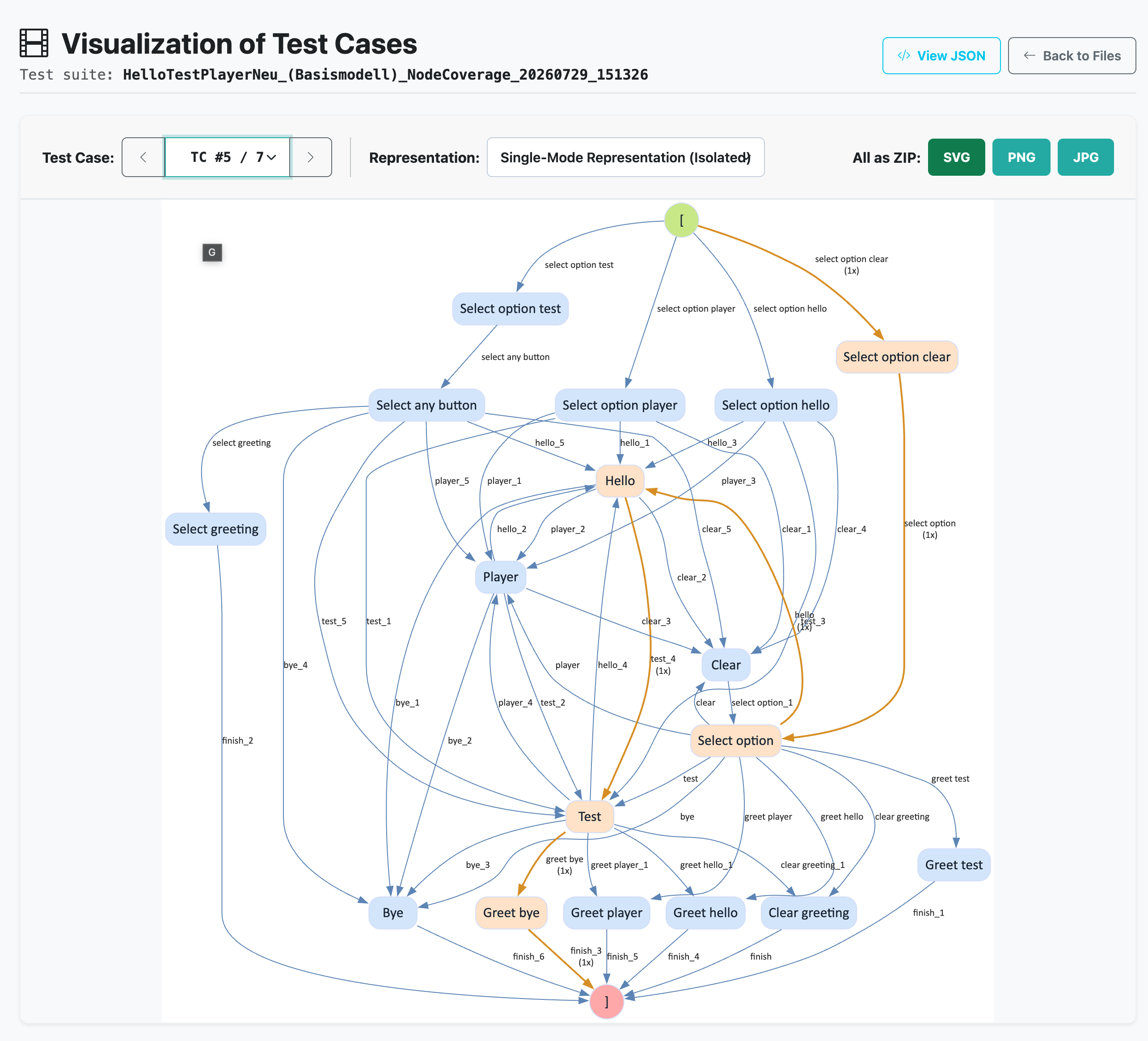
Figure 19 Single-Mode Representation of an individual test case.

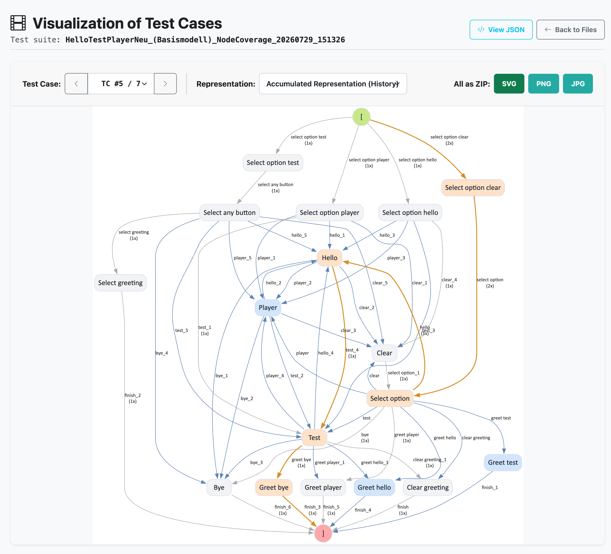
Figure 20 Accumulated Representation of a sequence of test cases.

8.2 Overview of the Test Suite (Test Focus)

The test focus aggregates all runs of a complete suite on a single graph. Edge thicknesses (penwidth 1 to 4) and colors (Matplotlib “Blues” palette) visualize the visit frequency, which is additionally displayed in the edge labels. Unvisited nodes and edges are grayed out and have no visit frequency.

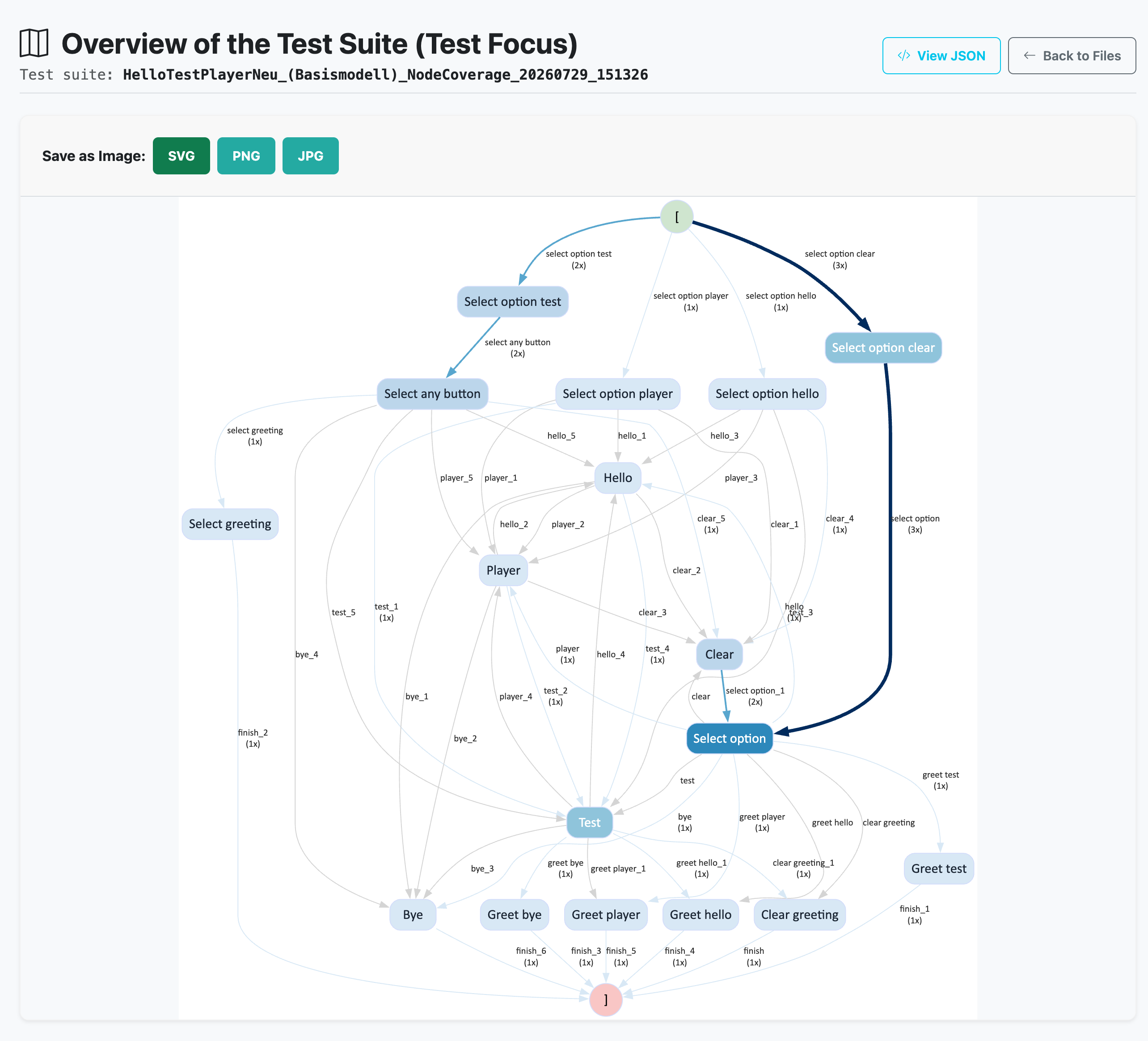
Figure 21 Test focus and visualization of the visit frequency.

8.3 Comparative Analysis (Overlays)

To analytically evaluate the quality of a generated test suite, the viewer offers an interactive comparison function (overlay) for the diagrams of the state and event frequencies. A second dataset (blue) can be overlaid on the current dataset (green) via the dropdown menu “⚖️ Compare with:”. Clicking the blue or green legend removes the blue or green dataset from the chart. Clicking again shows it again.

• Empiricism vs. Theory: Here, the empirically measured frequency of the test suite is compared with the theoretical steady-state probability of the MCUM base model to identify deviations of the random walk.

• Empiricism vs. Empiricism: Enables the direct comparison of two generated test suites with each other.

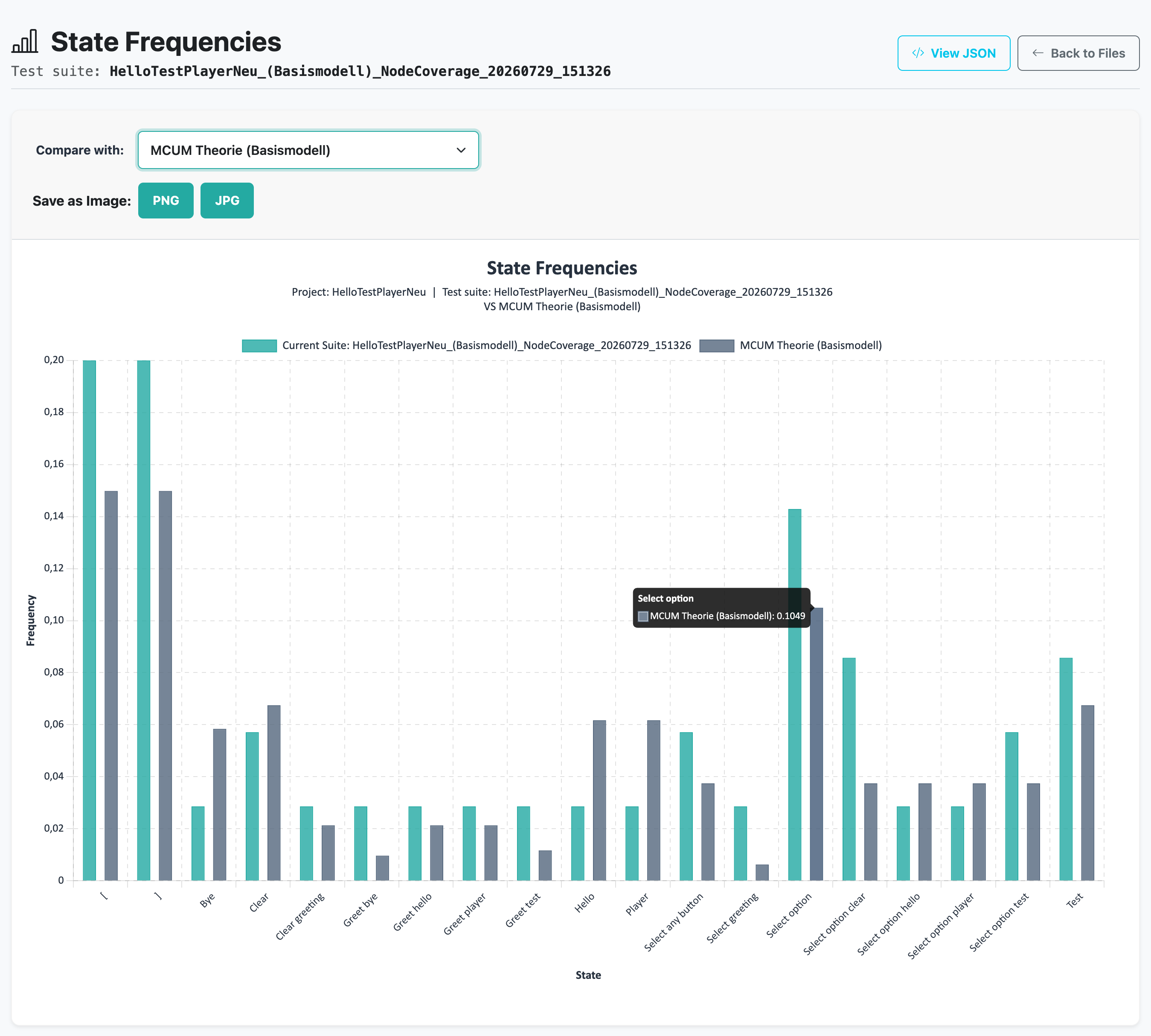
Figure 22 Comparison of a generated test suite with the theoretical MCUM probability.

Note

Efficiency increase through stochastic convergence: The overlay analysis provides the empirical proof for the “Law of Large Numbers” in Model-Based Testing. As can be seen in Figure Stochastic convergence: 1000 vs. 250 test cases in direct comparison., the distribution of a gigantic test suite (e.g., 1000 test cases) differs only asymptotically from a significantly smaller suite (e.g., 250 test cases). The effort for the subsequent test execution can thus be drastically reduced in practice (e.g., to a quarter) without suffering serious losses in accuracy in the profile coverage.

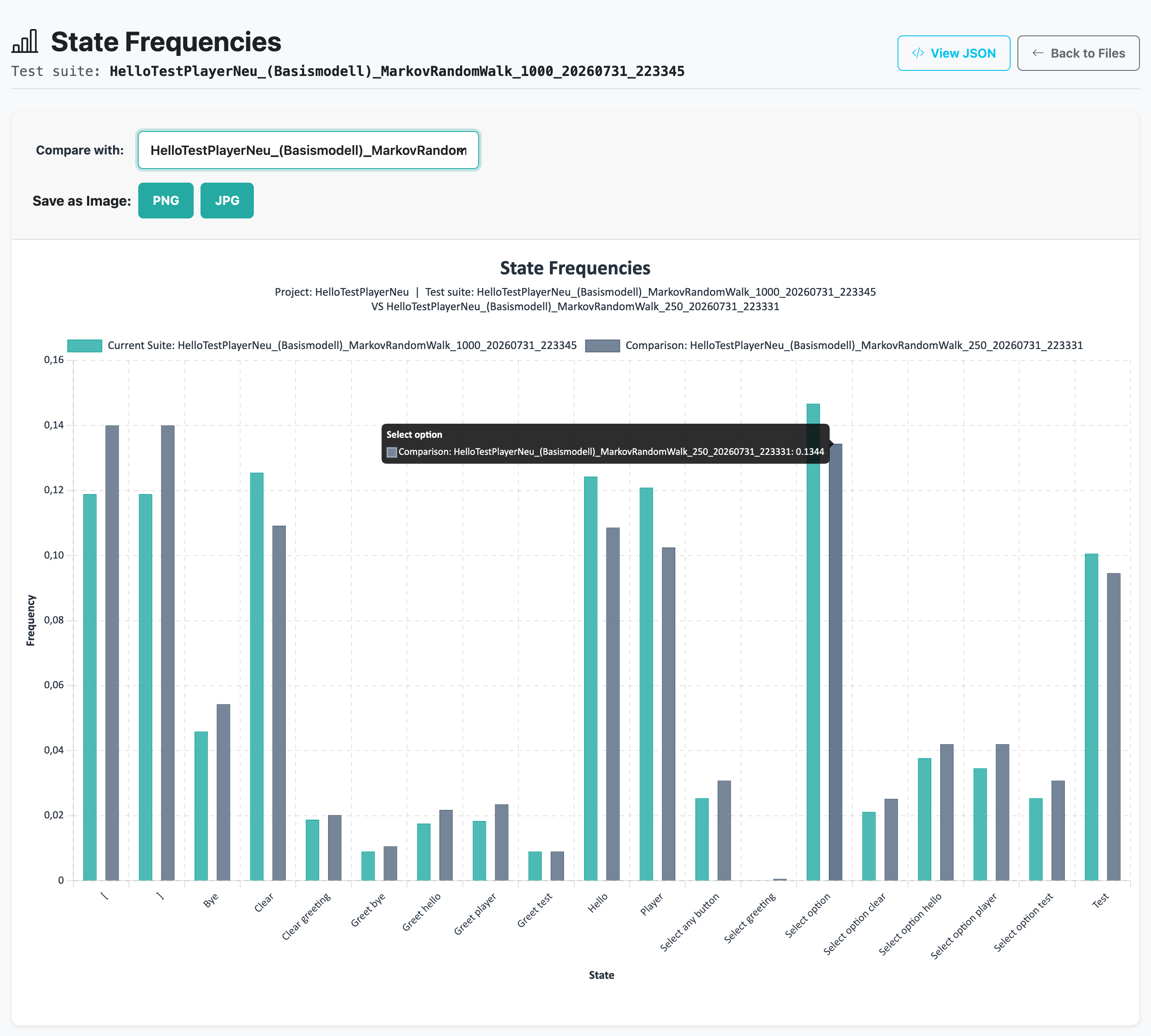
Figure 23 Stochastic convergence: 1000 vs. 250 test cases in direct comparison.

9. Execution and Performance Visualization of Test Runs

As soon as a test suite has been executed against a System Under Test (SUT), two further phases (Phase 3 & Phase 4) are available in the workspace for detailed performance evaluation. These views visually implement the metrics from Smart Testing 2.0 [1].

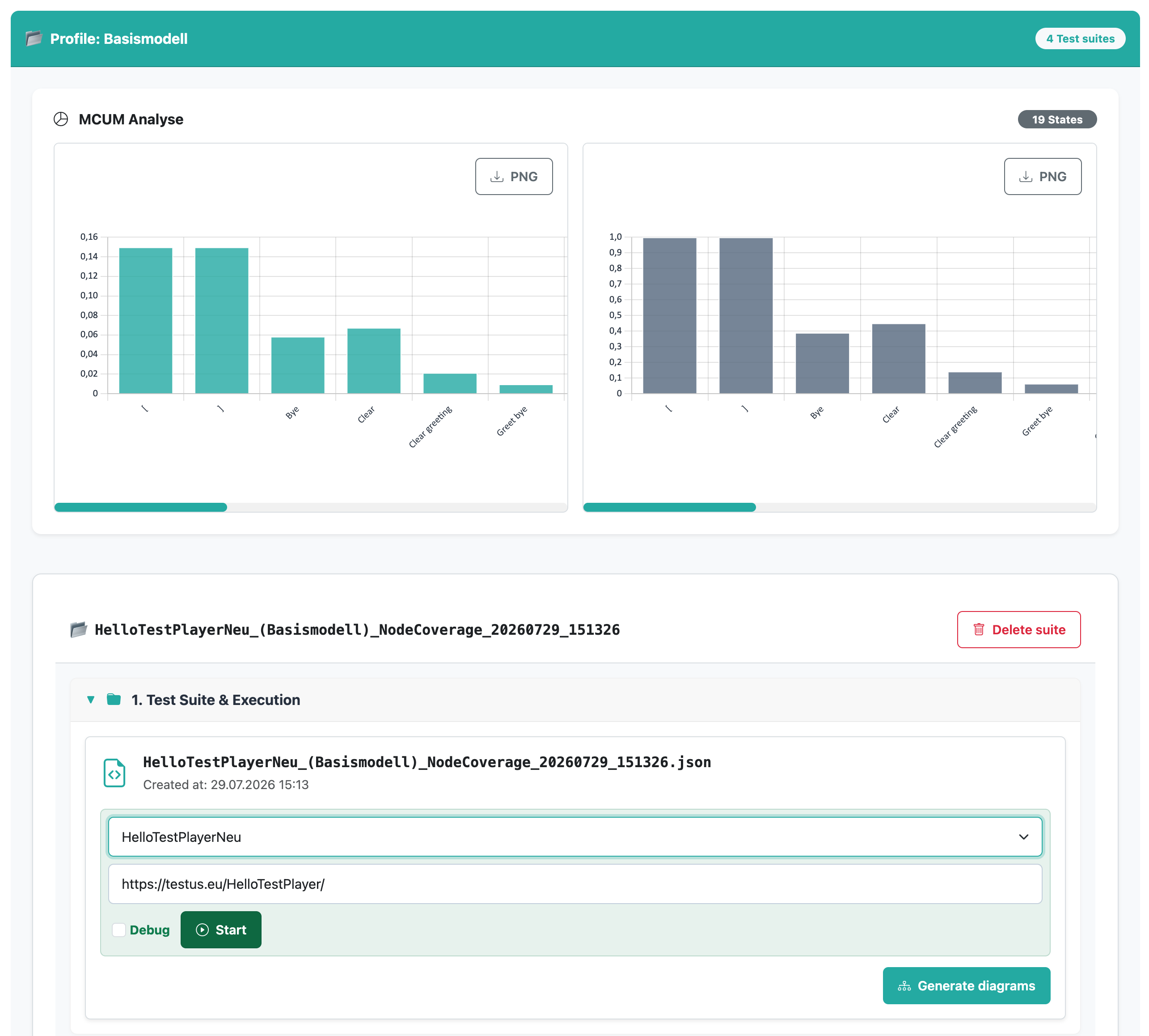
Figure 24 Starting a test run.

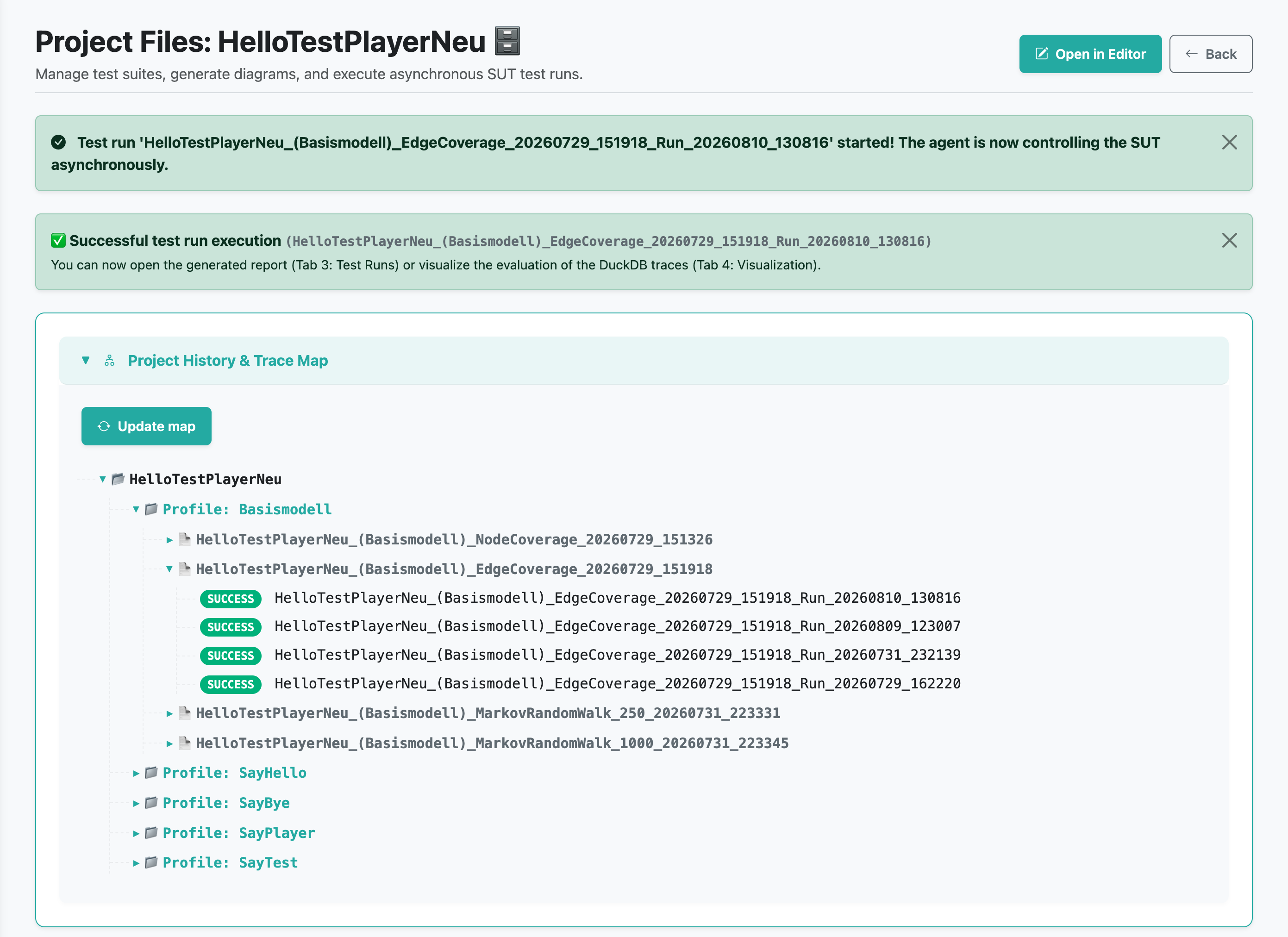
Figure 25 Successful progress of the test run.

9.1 Test Runs (Reports & DuckDB Live-Traces)

This section provides the raw data and an aggregated summary of the selected test run:

• Overview cards: Show the execution time window, the total duration in ms, the real test execution time (including operating system overhead for starting/stopping the asynchronous Playwright agent and saving the trace data in the database), the number of evaluated test cases and test steps, as well as a status matrix (PASS / FAIL / ERR).

• Overview charts: Two diagrams provide information on the absolute frequency and the execution times of individual test steps of the test run.

• Breakdown of test cases: An expandable accordion with which each test case and the results of its individual test steps can be inspected chronologically.

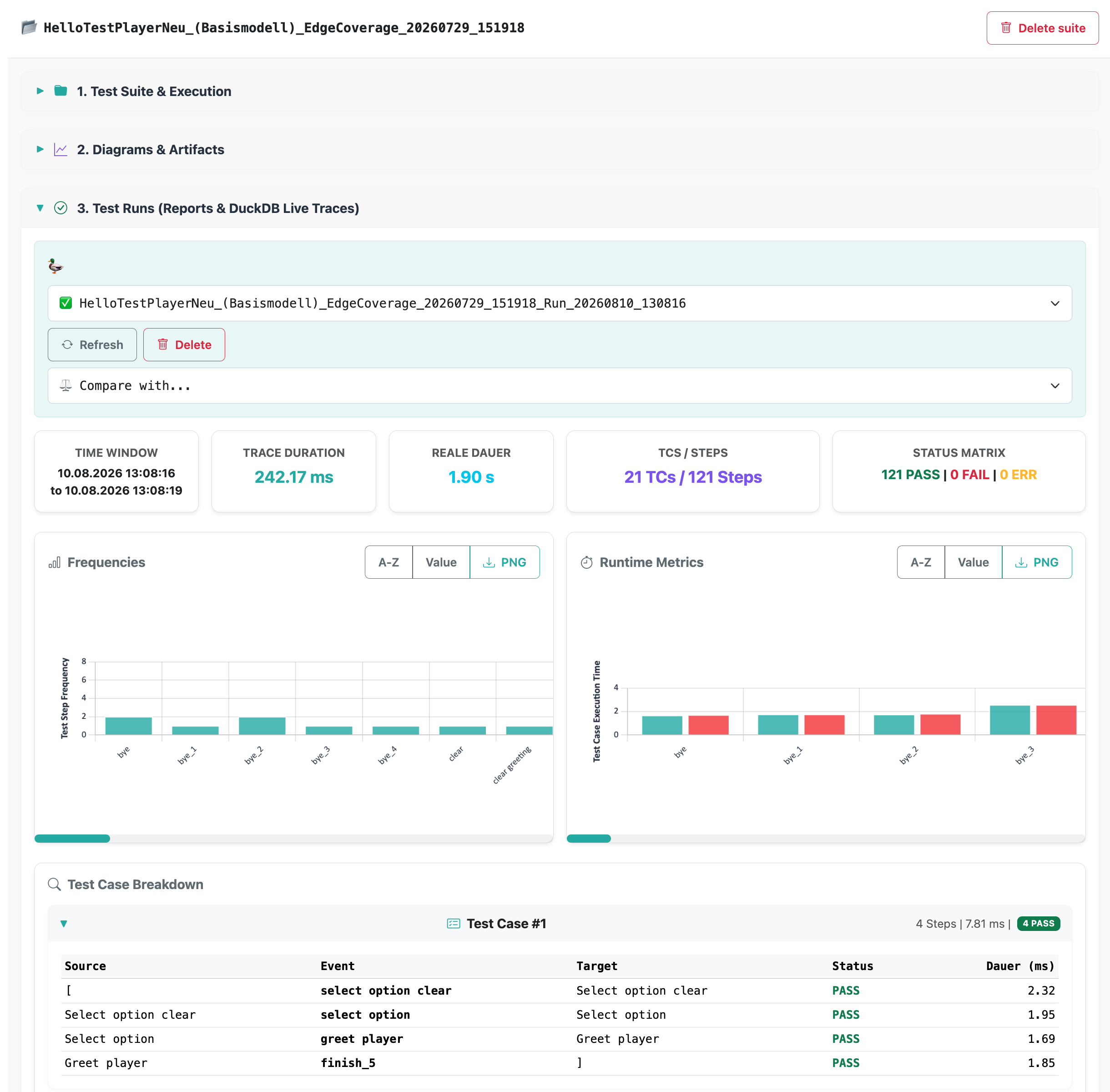
Figure 26 Execution time window, the total duration, the number of evaluated test cases and steps.

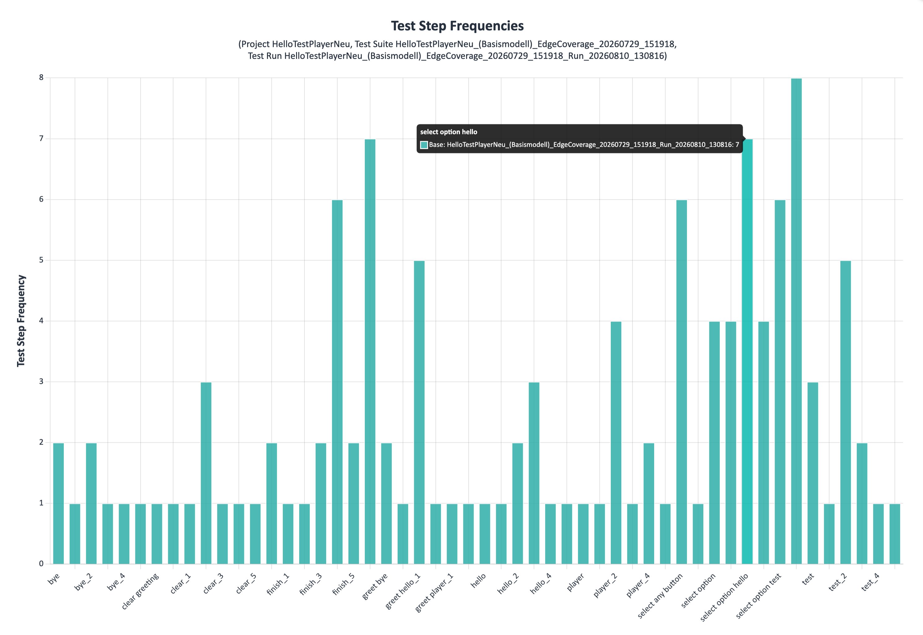
Figure 27 Absolute frequencies of individual test steps.

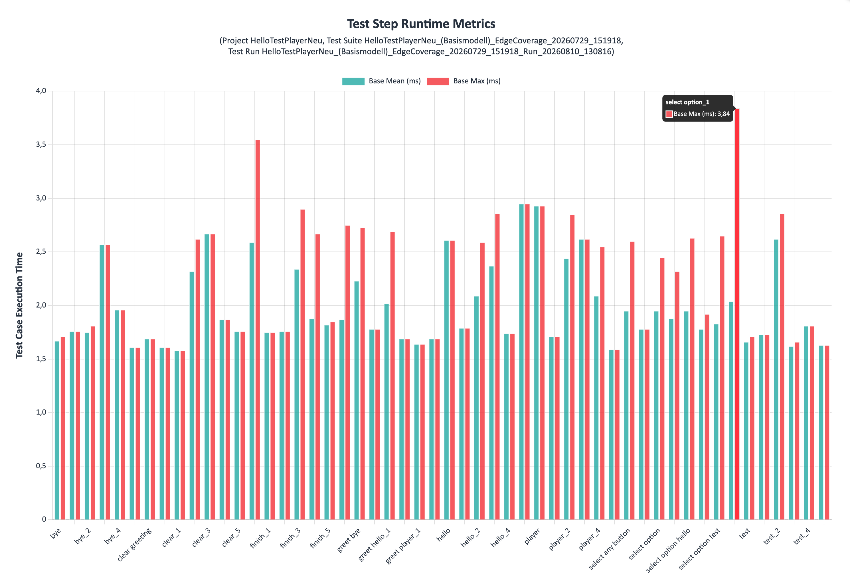
Figure 28 Processing times of the individual test steps.

9.2 Visualization of the Test Runs (Performance Metrics)

The fourth phase offers in-depth diagrams for identifying bottlenecks in the SUT. Clicking on a diagram opens it in a high-resolution lightbox view (zoom), whereby the proportions and font sizes are dynamically preserved [3]. All axes support Natural Sorting, whereby labels like e2 are mathematically correctly sorted before e11 [3].

• Execution Times of the Complete Test Suite: A timeline that visualizes the runtime of every single executed step of the entire suite.

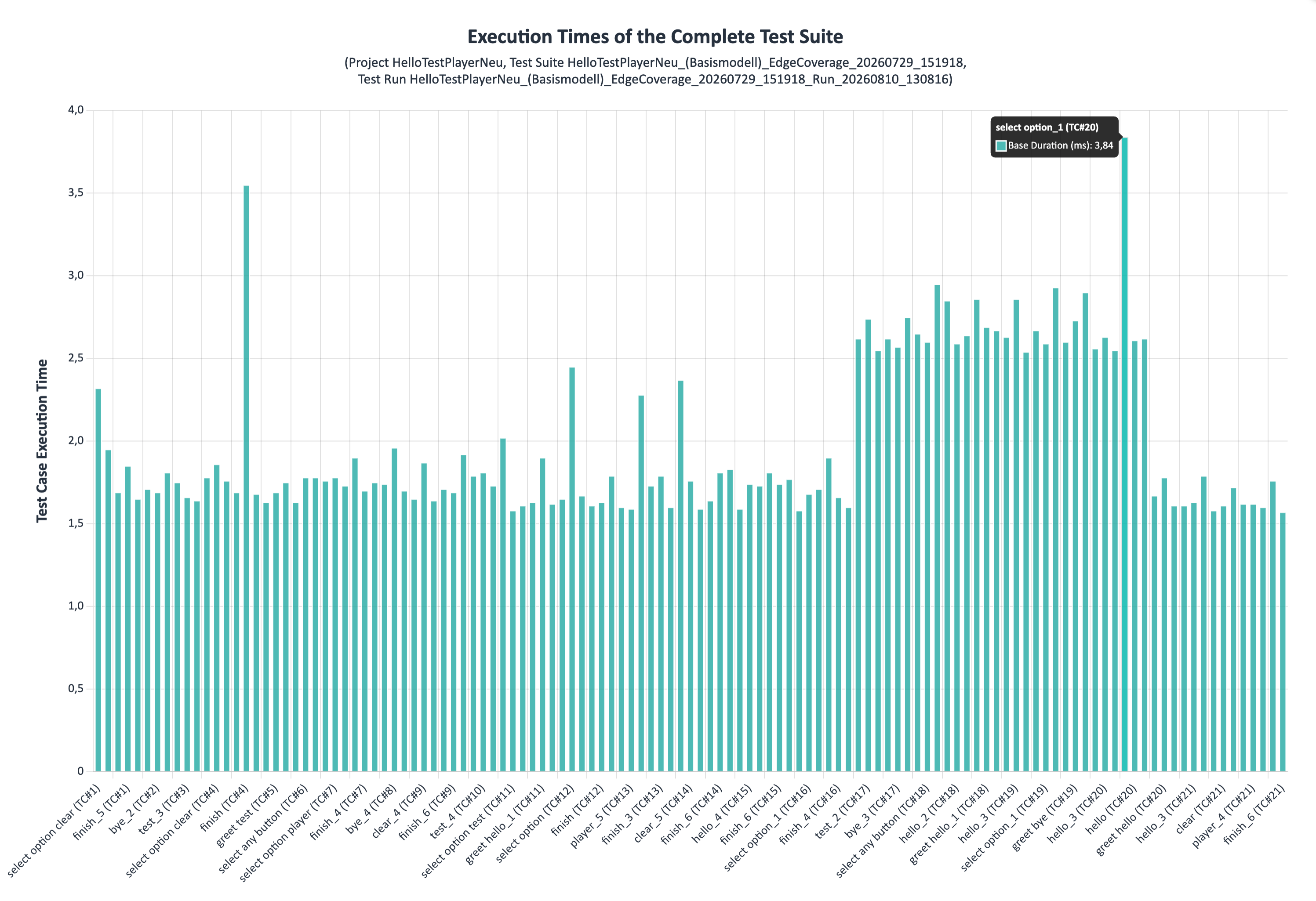
Figure 29 Representation of the execution times of a complete test suite.

• Execution Times for Test Case: An isolated timeline for a specific test case, which can be selected from a dropdown menu.

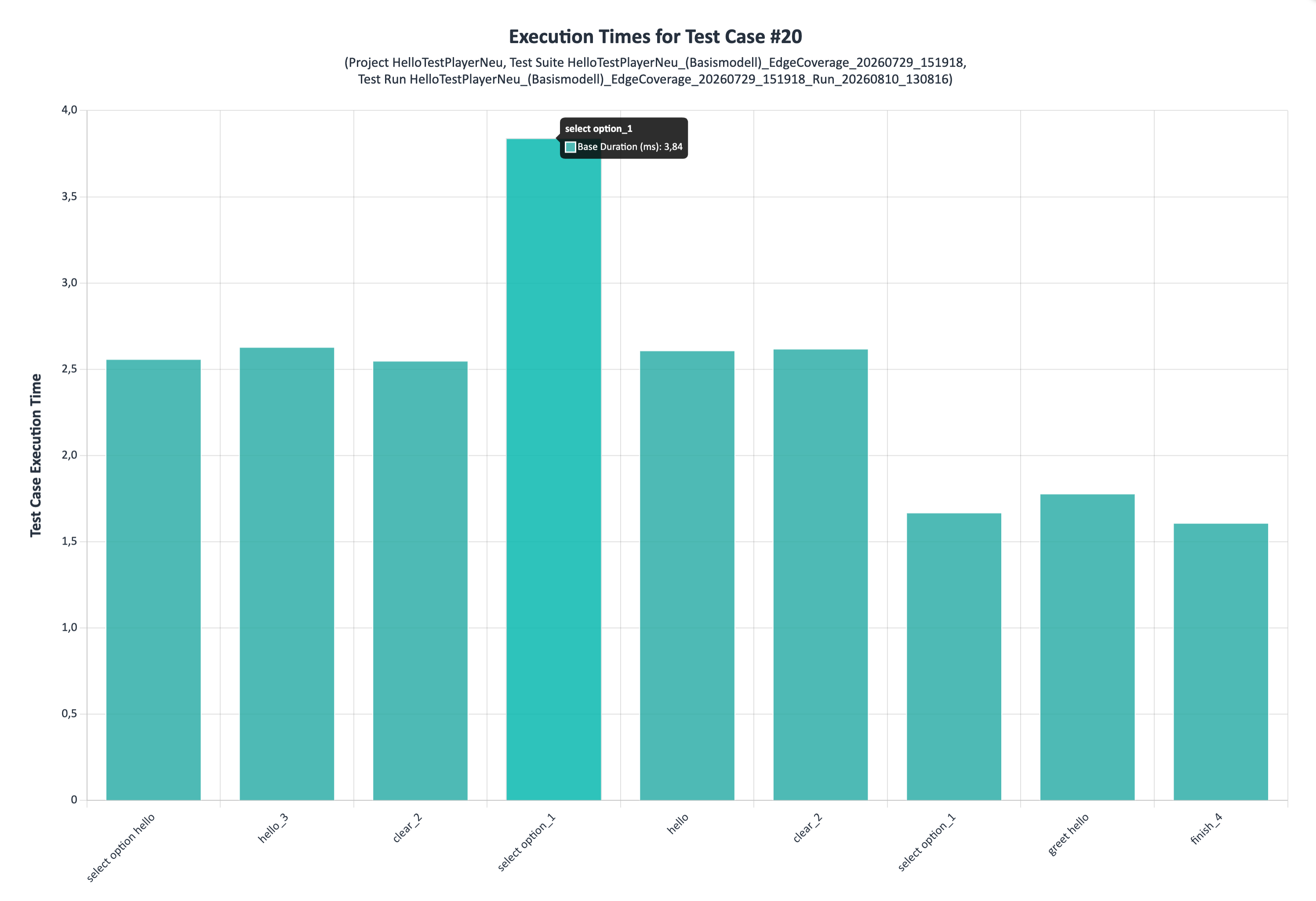
Figure 30 Representation of the execution times of an individual test case.

Detailed metrics on the execution of individual test steps:

To uncover outliers in application performance, the execution times of all identical test steps are aggregated and evaluated:

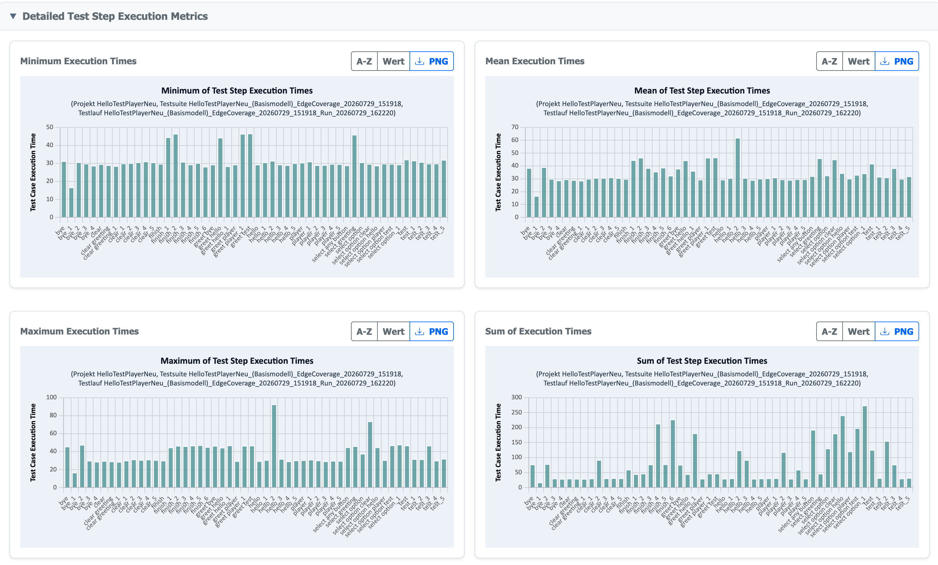
Figure 31 Detailed metrics on the execution of individual test steps.

• Minimum Execution Times: Shows the fastest execution time of a test step over the entire test run (best-case scenario).

• Mean Execution Times: Calculates the average runtime and serves as a robust indicator for regular system performance.

• Maximum Execution Times: Highlights outliers where a single step took an untypically long time (worst-case scenario).

• Sum of Execution Times: The cumulative total execution time reveals which steps aggregated consumed the most computing time of the test run.

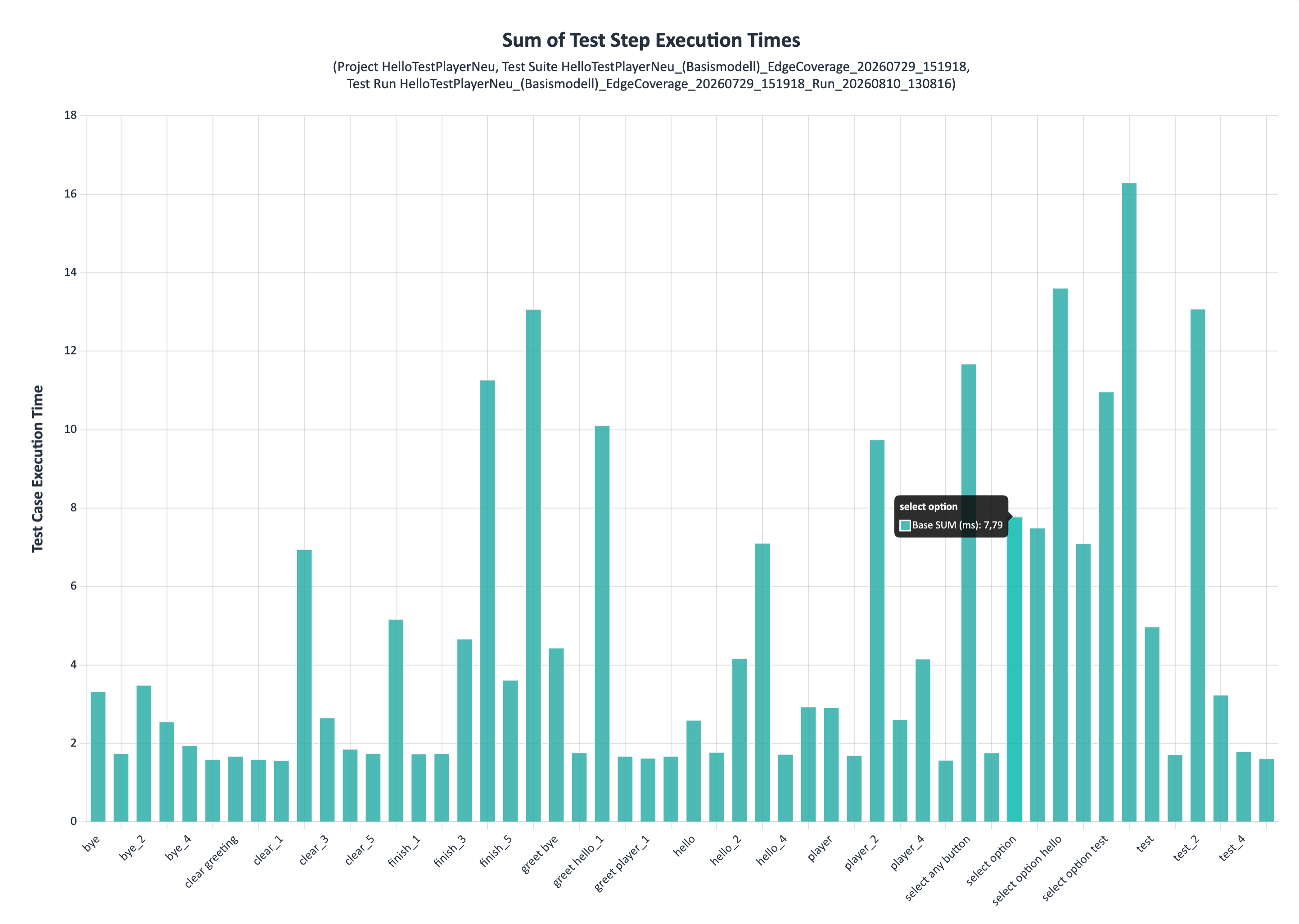
Figure 32 Cumulative total execution time of individual test steps.

9.3 Comparative Performance Analysis (Overlays)

Analogous to the structural comparison of test suites, the empirical metrics of two independent test runs can also be superimposed directly on each other. Via the dropdown menu “⚖️ Compare with:”, a second test run (gray bars) can be overlaid on the base run (turquoise bars).

• Dynamic Union Set: If a run terminates prematurely (e.g., due to an error), the system automatically interpolates the X-axis over the maximum length of both runs. Missing events are left on the axis and filled with zero values, so that the chronological representation and the comparison remain absolutely synchronous.

• Identification of Regressions: The overlaid bar charts make performance drops between two test iterations, code refactorings, or different SUT releases visible at a glance.

As can be seen, the second test run shows significantly higher values for execution times. This can occur when there is a higher volume of background traffic or when many parallel tasks happen to affect the execution time of the test run.

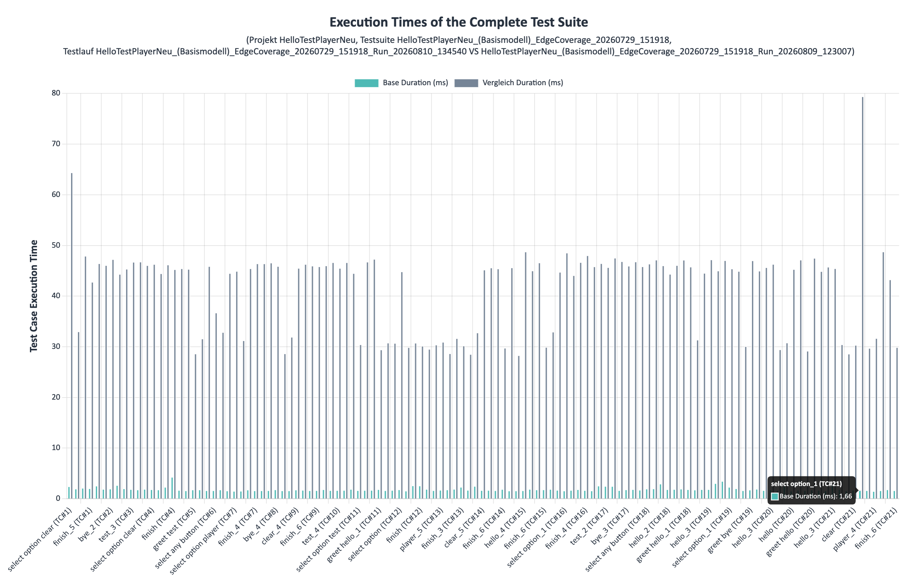
Figure 33 Comparative Performance Analysis: Comparison of the execution times of two test runs.

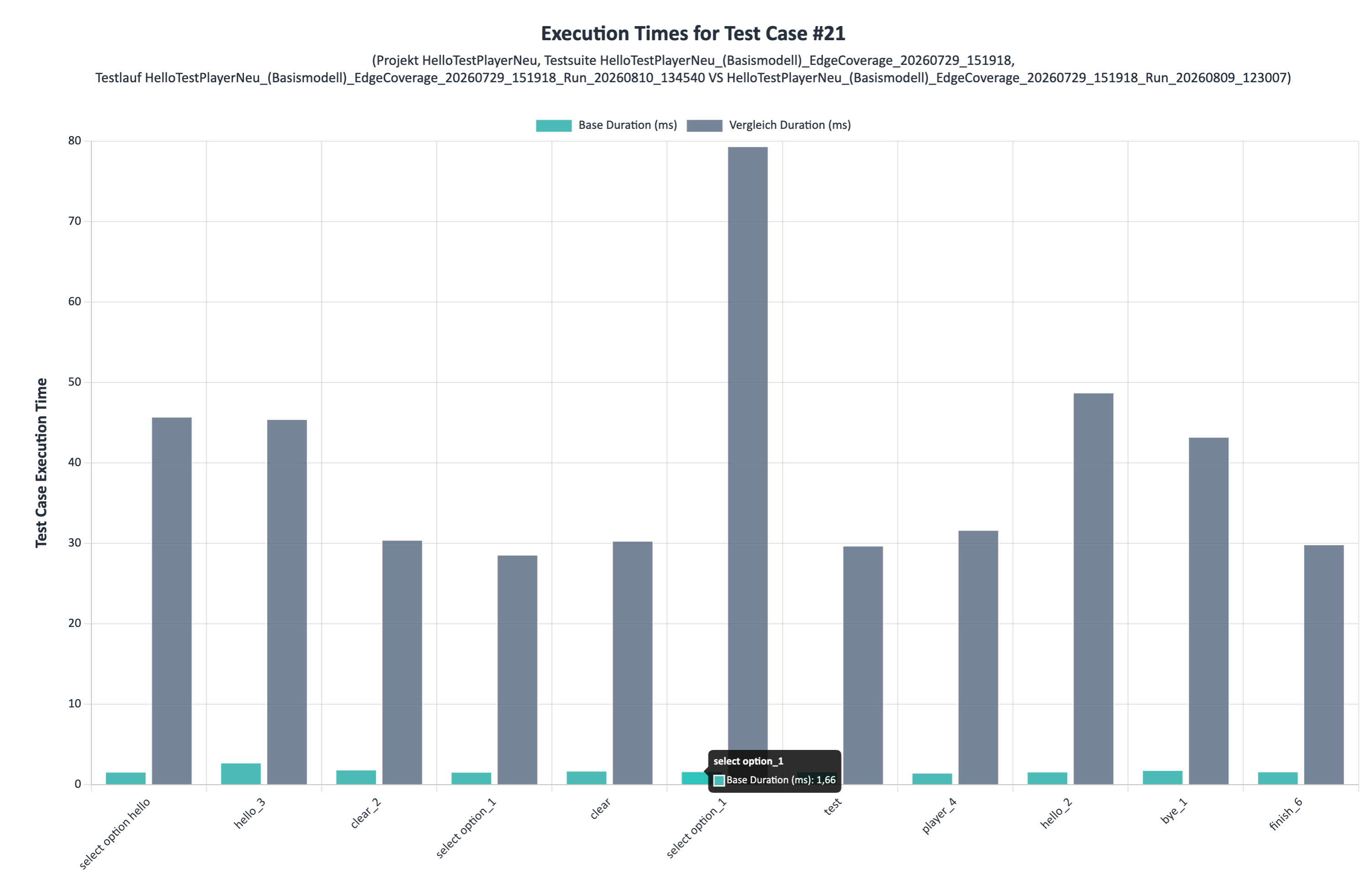
Figure 34 Comparison of the execution times of two test cases.

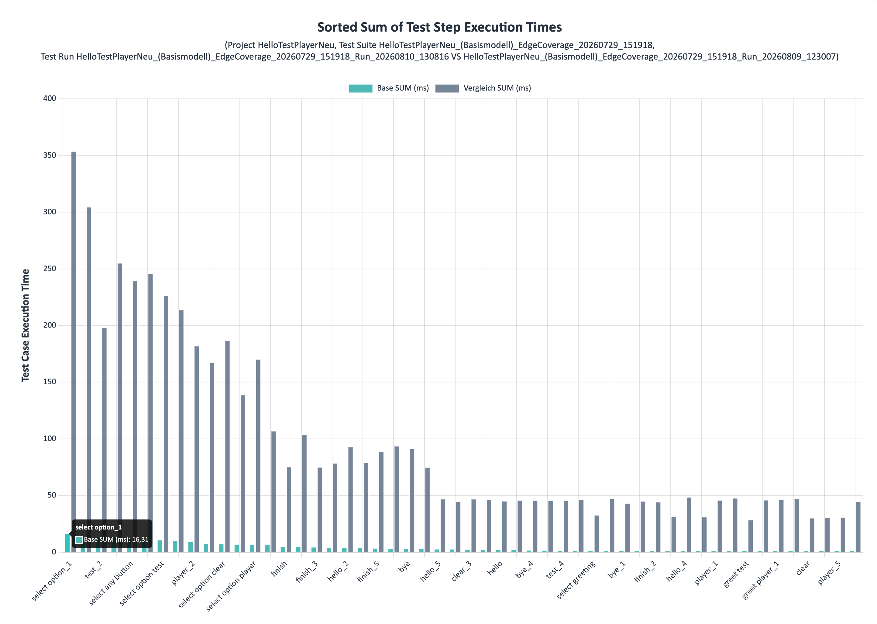
Figure 35 Sorted comparison of the sum of the execution times of two test runs.

9.4 Playwright Replay (Video Recording)

To be able to analyze not only the static DOM state (trace) but also the dynamic progression of failed test runs, TestPlayer 2.0 offers a complete video recording of the browser session. If a test suite is started with the Debug mode via the checkbox before execution, the Playwright Automation Engine records the entire interaction as a compressed .webm video.

This replay enables the tester to dynamically view the exact User Journey, layout shifts, and animations exactly as the agent experienced them at runtime. The video is automatically linked to the corresponding test run record (TestRun) and can be used for error analysis.

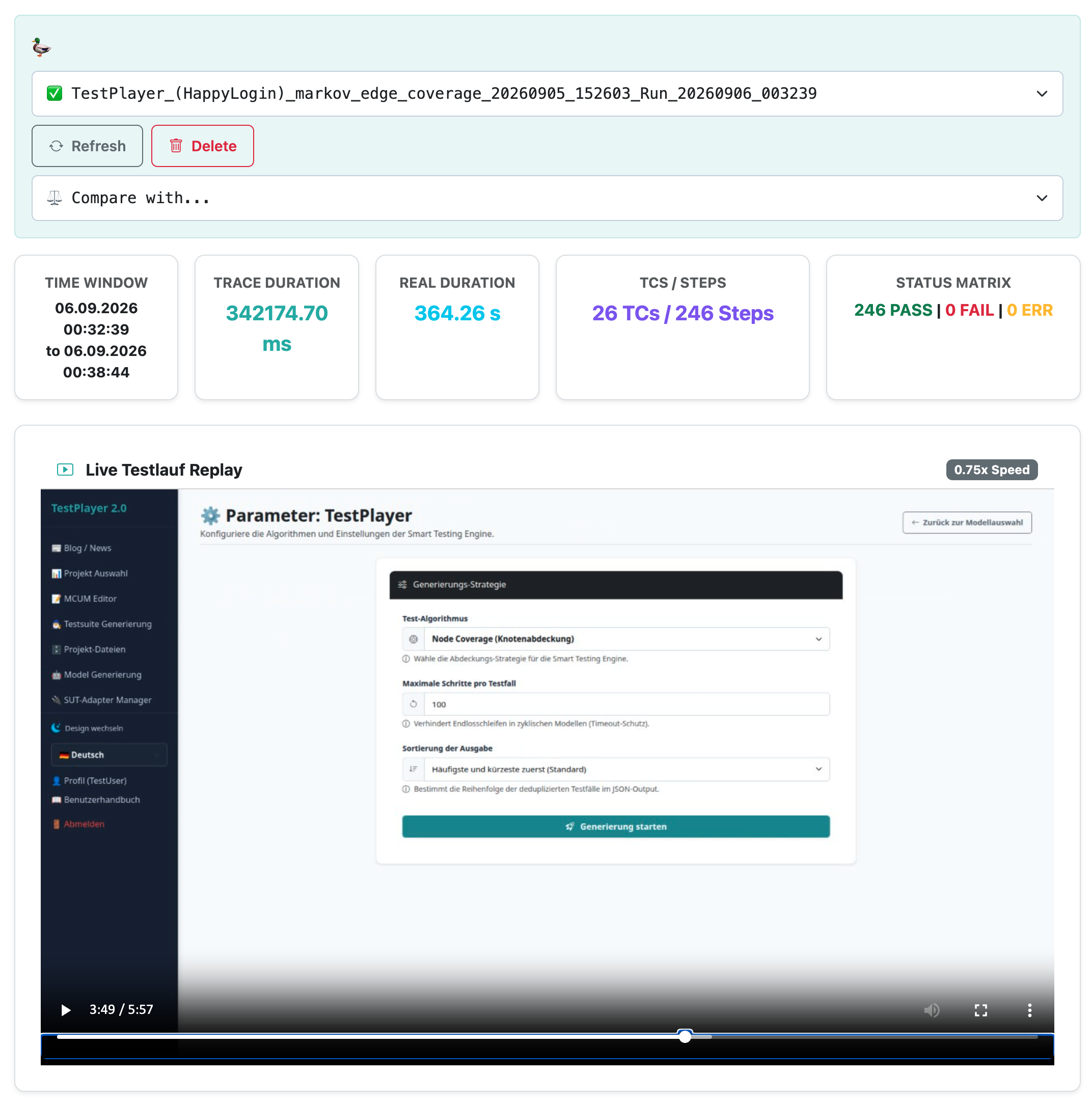
Figure 36 Playwright Replay: Complete video recording (.webm) of an asynchronous test run in debug mode.

10. Export Functions

All diagrams and graphics can be exported for external documentation and reports:

• Statistics & Metrics: Direct individual download as .png or .png. The diagrams contain a dedicated book layout (Calibri, bold two-line subtitle and blue background) and automatically receive unique filenames [3].

• Test Case Frames: Batch export. The Diagram Viewer renders all frames asynchronously in the background and bundles them as a named .zip archive.

11. Auto-Discovery of MCUMs (Automated Model Generation)

The manual creation of state transition models for complex web applications is time-consuming and error-prone to UI changes. To resolve this bottleneck, TestPlayer 2.0 features an integrated Auto-Discovery Engine. This functionality allows the System Under Test (SUT) to be explored automatically (crawling) and a valid Markov Chain Usage Model (MCUM) in DOT format, as well as an initial SUT adapter, to be generated from it on-the-fly.

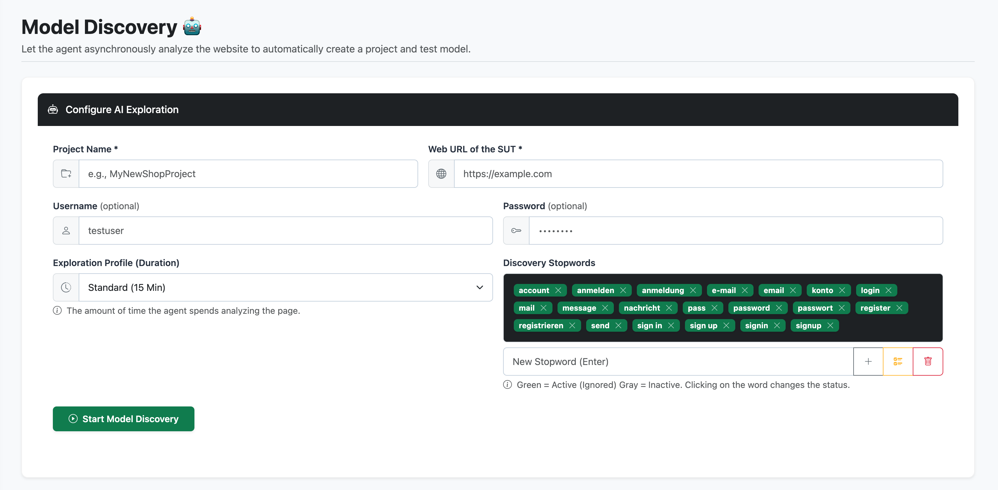
Figure 37 Auto-Discovery of MCUMs.

11.1 Configuration and Stopword Filtering

Before the exploration begins, the user configures the target SUT and the desired duration of the exploration profile (e.g., 5 to 60 minutes) via the Model Discovery user interface. To prevent a state-space explosion and keep the generated model strictly focused on the relevant business logic, the system features a dynamic Discovery Stopwords tag system.

Users can explicitly add, toggle, or remove specific keywords (e.g., “login”, “password”, “register”) here. During the crawling process, the Vision-LLM is strictly instructed to ignore any UI elements or actions that match these active stopwords. This reliably prevents the autonomous agent from getting caught in authentication loops or exploring irrelevant administrative sections of the application.

11.2 How Exploration Works (UI Crawling)

The Auto-Discovery Engine uses a headless Playwright agent that independently interacts with the target application. The process iteratively passes through the following phases:

1. Initialization: The agent navigates to the start URL and analyzes the Document Object Model (DOM) of the current view.

2. Action Extraction: A heuristic parser identifies all interactable elements (buttons, links, input fields, dropdowns) on the current page.

3. Execution & Tracing: The agent selects an action (e.g., a click), executes it, and waits for the subsequent page to render to ensure that the view is fully loaded.

4. Graph Building: The origin state, the executed action (edge), and the newly reached state are logged in a dynamic graph structure.

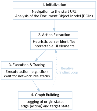
Figure 38 Phases of Auto-Discovery: From the initial page visit to dynamic Graph Building.

11.3 State Abstraction

The greatest challenge in automatic model generation is recognizing whether the application is in a new or a previously known state after an action. For this purpose, TestPlayer 2.0 uses intelligent state abstraction:

• DOM Hashing: Instead of comparing the entire HTML structure, the engine extracts structure-giving features (e.g., the number and type of containers, active navigation elements, form fields) and generates a unique hash value from them.

• Dynamic Data Ignorance: Fluctuating content such as times, random IDs, or temporary advertising banners are excluded from the hash by the filter rules to prevent state explosion.

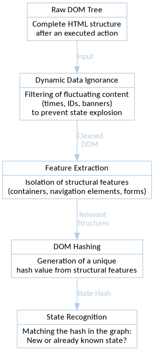
Figure 39 State abstraction: Filtering dynamic UI elements to generate robust State Hashes.

11.4 From Exploration to Markov Model (MCUM)

After exploration (e.g., via a defined time limit or a set node coverage) is completed, the graph is available as a topological ground truth. In the last step, this graph is transferred into a stochastic model (MCUM).

The empirical probabilities of the edges (transitions) are calculated based on the observed frequencies during crawling. The probability \(p\) for the transition from state \(s_i\) to state \(s_j\) upon executing action \(a\) is determined by:

\[p(s_i \xrightarrow{a} s_j) = \frac{n(s_i, a, s_j)}{\sum_{k} n(s_i, a_k, s_k)}\]

Where \(n\) represents the absolute number of observed traversals. Edges that lead to errors (e.g., 404 pages or infinite loops) can be automatically penalized with penalty probabilities or marked as isolated error nodes. The final model is exported in DOT format and is immediately available in the dashboard for test case generation.

11.5 Synergy with the SUT Adapter Lifecycle

The DOT model generated by Auto-Discovery naturally possesses machine-generated (structural) locators, such as long and unreadable CSS paths (div > span:nth-child(3) > button).

This is exactly where the transformation workflow comes into play (see Administration Manual, Chapter 3.2): The script transform_adapter uses heuristic matching to fuse the freshly discovered, accurate topology of the auto-discovery with the human-readable, semantic names (e.g., btn_login) of a manually maintained reference adapter. In this way, a test model is fully automatically created that is 100% structurally equivalent to the current application and at the same time offers readable, maintainable UI locators for the Smart Testing Engine.

12. Case Study: Automatic Discovery and Generation for the “Playwright” Project

This overarching end-to-end case study demonstrates the complete workflow of TestPlayer 2.0 in practice. The official documentation site of the Playwright Automation Engine serves as the test object.

12.1 Initialization and Auto-Discovery

The process begins without an existing DOT model. Instead, the Auto-Discovery Engine (see Chapter 11) is started with the target URL of the Playwright website. The agent navigates the site autonomously, identifies interactable elements in the DOM, and iteratively builds a graph.

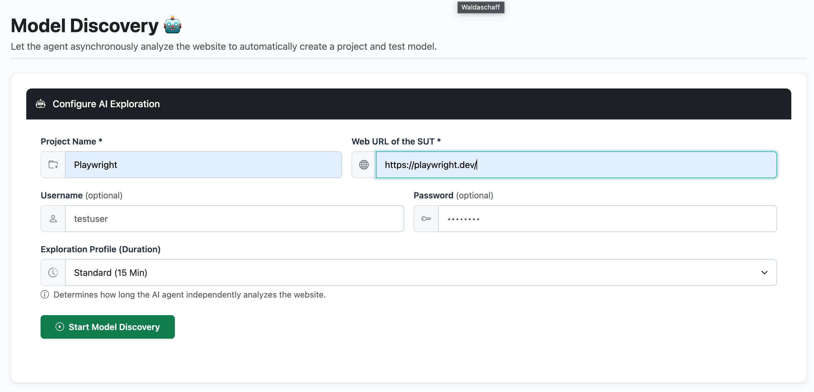
Figure 40 Step 1: Configuration and start of the auto-discovery run on the target system.

After completion of the exploration phase, the system converts the collected metadata into a valid Markov Chain Usage Model (MCUM). The result is a topological “ground truth” of the Playwright documentation, where navigation paths, states, and edges (events) were automatically derived.

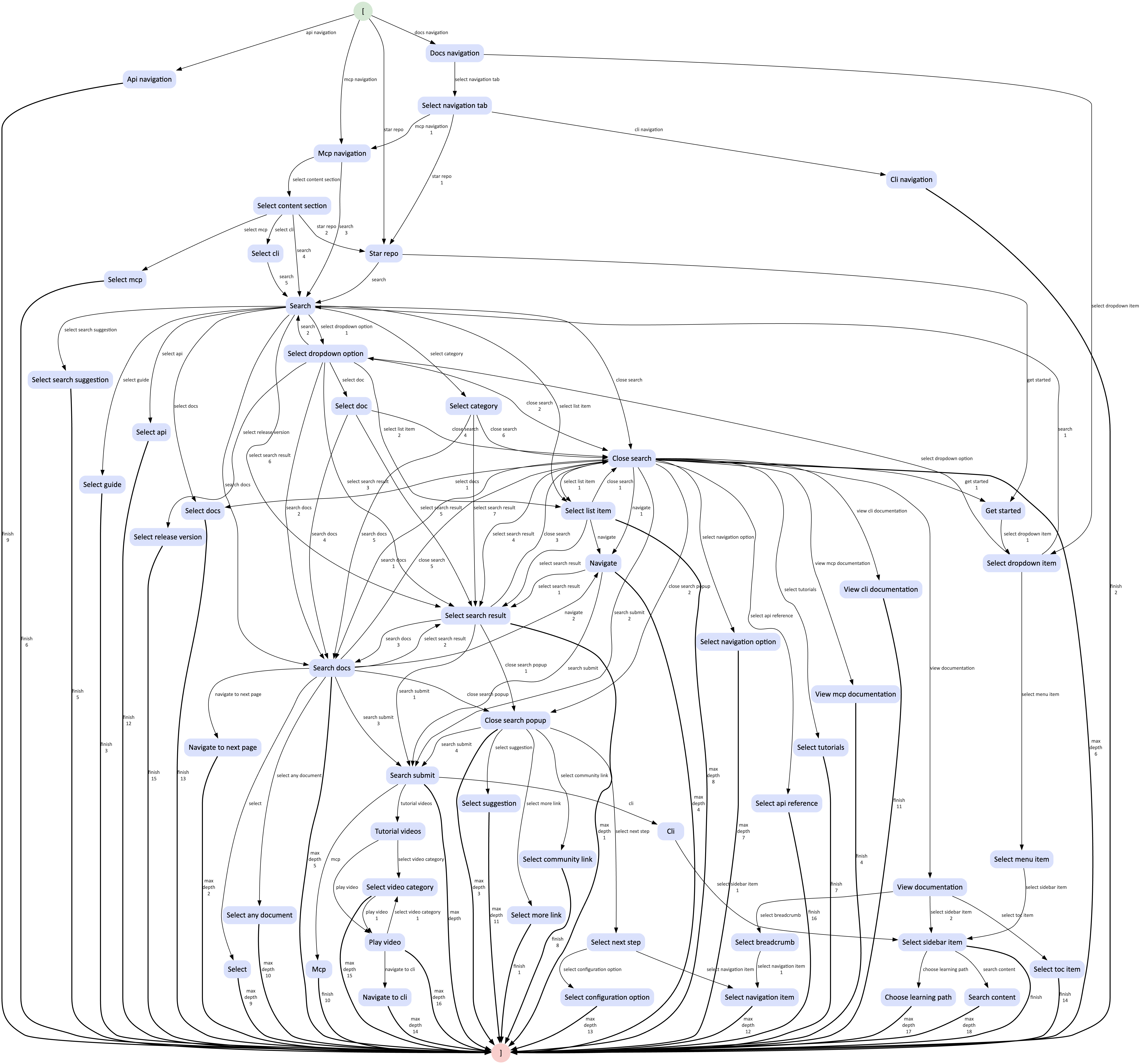
Figure 41 Step 2: The state transition model automatically generated from the exploration.

12.2 Project Workspace and File Management

As soon as the model is saved, TestPlayer 2.0 automatically creates a new project workspace. The newly discovered base model, including the profile structure, is stored here.

12.3 Test Suite Generation via the MBT Wizard

Using the model as a basis, the MBT Wizard is now started to calculate an executable test suite. In this scenario, the algorithm for Node Coverage is selected to ensure that every usage state found by the discovery is traversed at least once during the test run.

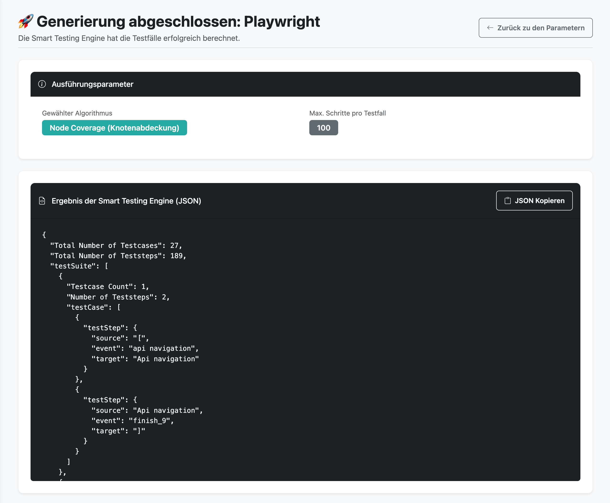
Figure 42 Step 3: Generation of a test suite for the state coverage of the SUT.

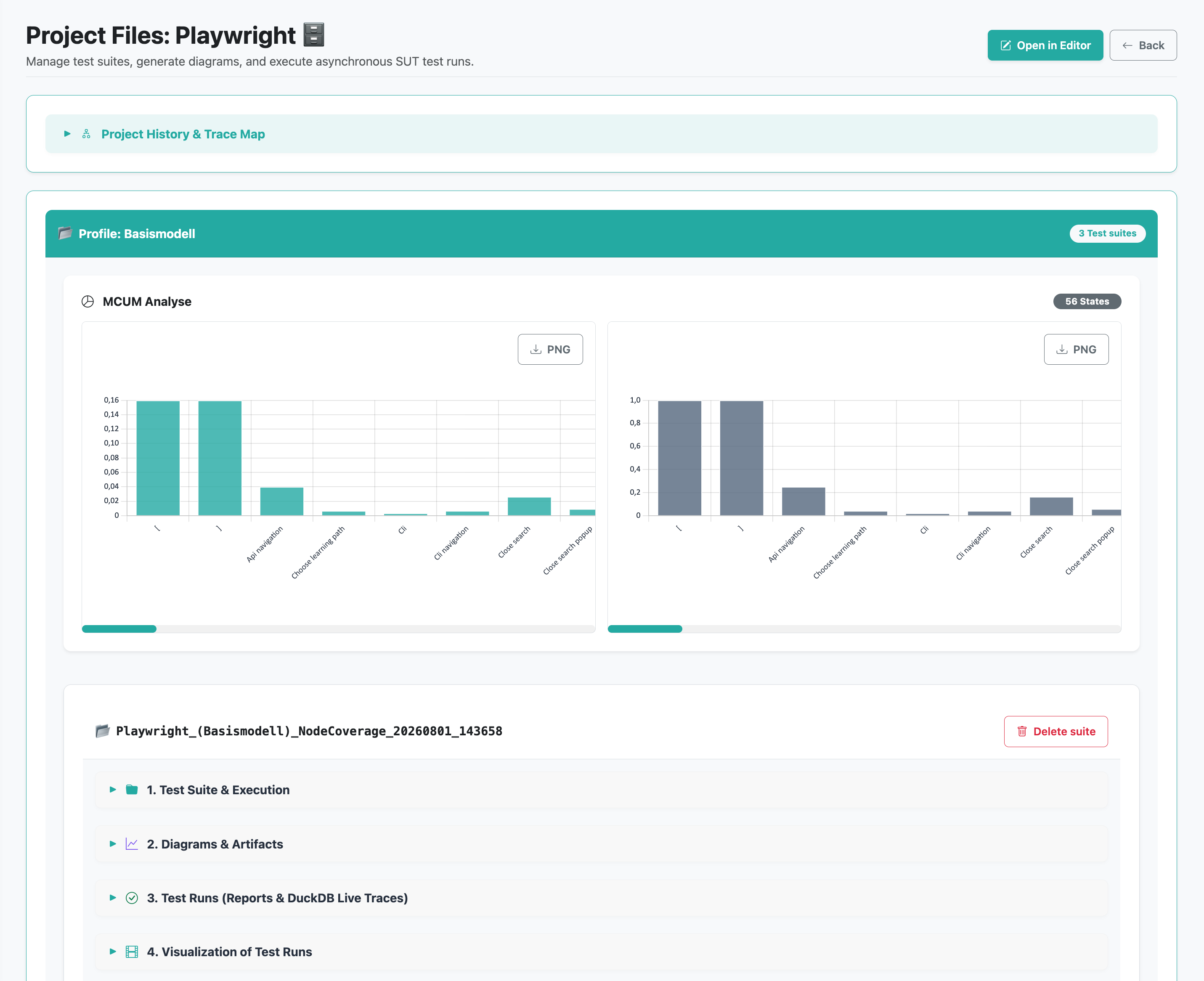
Figure 43 Step 4: The hierarchical workspace of the new test suite.

12.4 Visual Inspection (Diagram Viewer)

Before the asynchronous test run is started against the real SUT, the calculated suite can be reviewed in the Diagram Viewer. Here, it can be visually validated which paths the algorithm has chosen through the auto-discovery model.

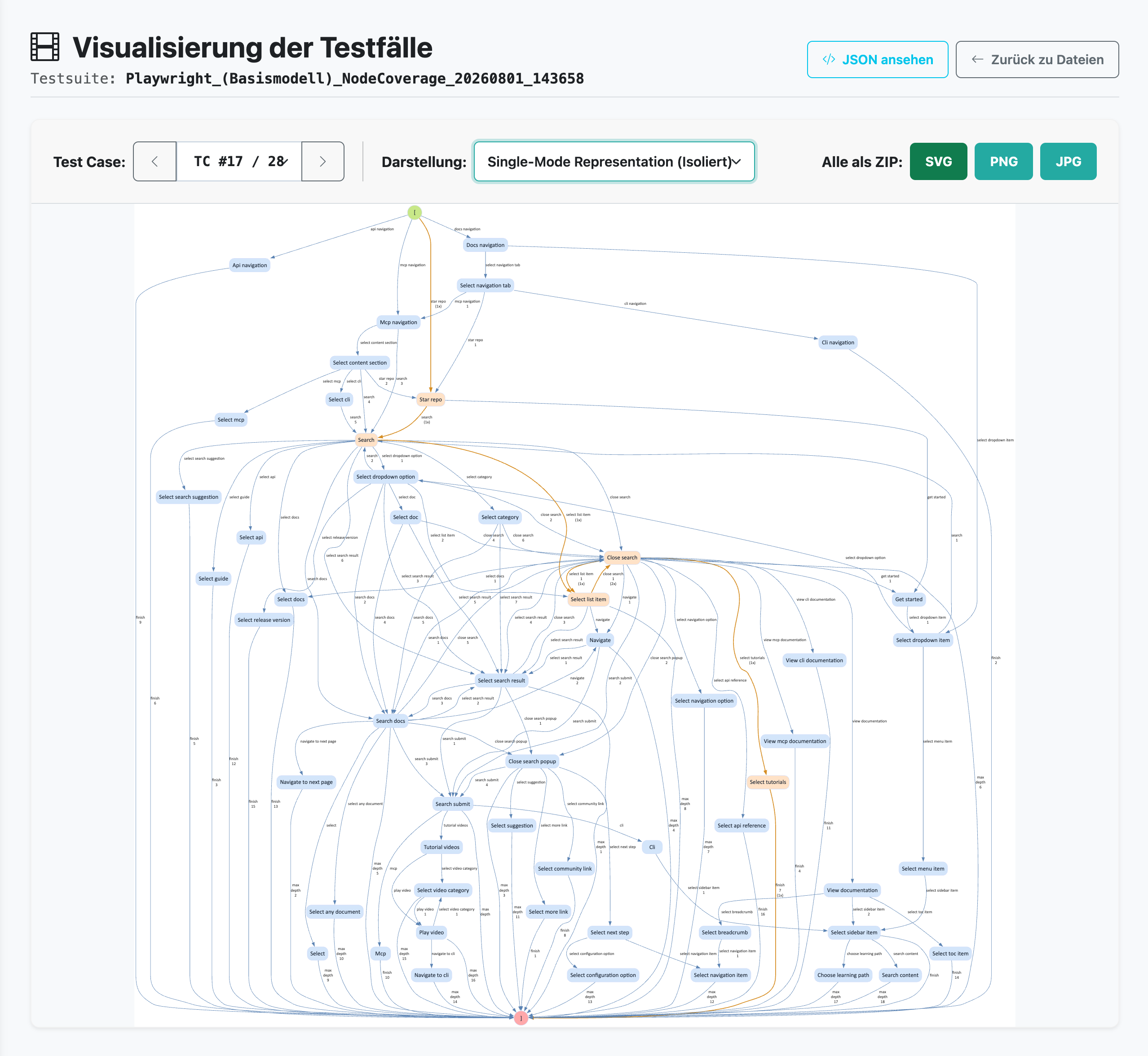
Figure 44 Step 5a: Inspection of an individual, generated test case (Single-Mode).

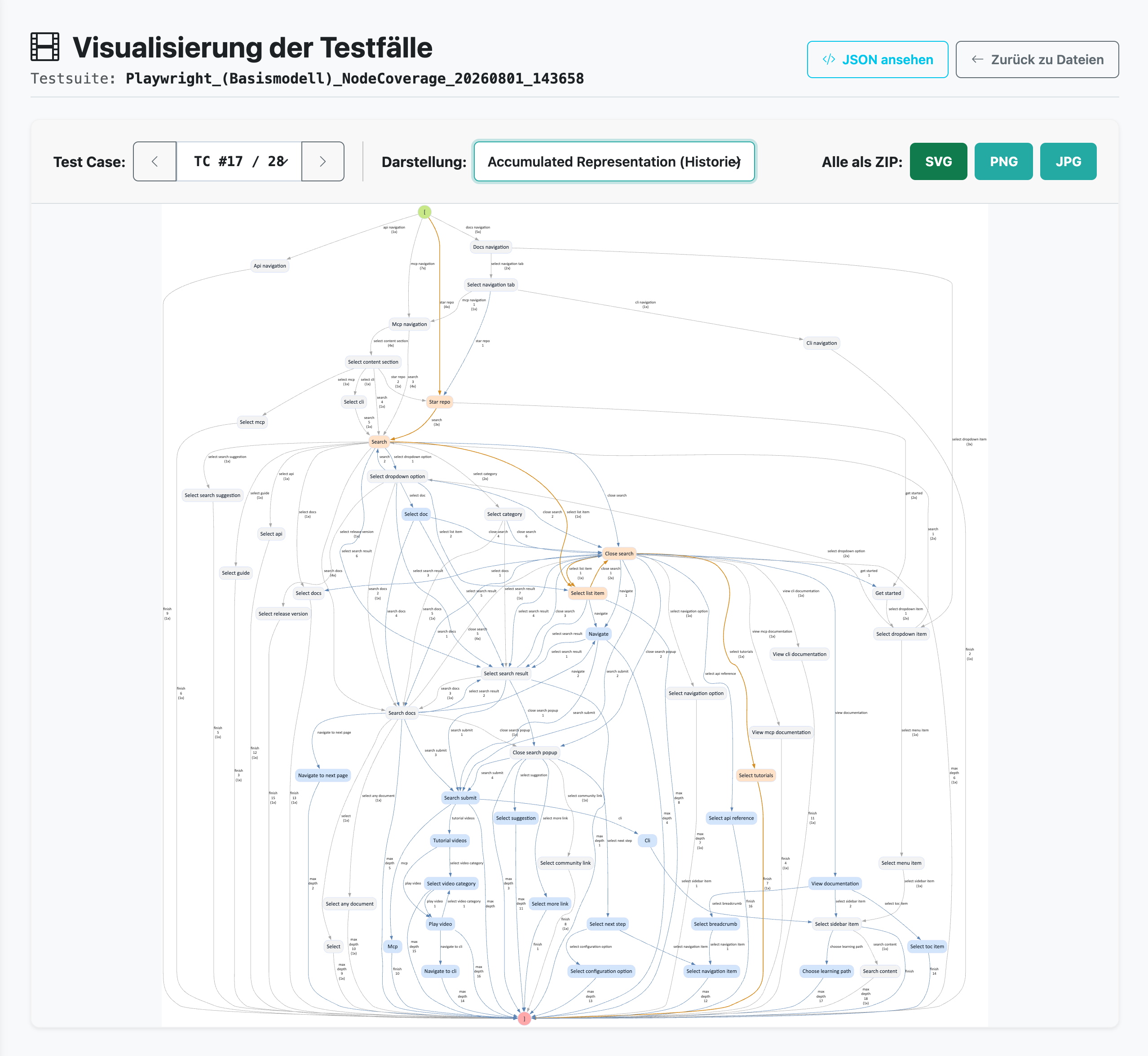
Figure 45 Step 5b: Verification of the growing state coverage (Accumulated Representation).

The aggregated test focus confirms that the goal of node coverage has been achieved: All states have been covered, and the color heatmap (Blues palette) illustrates the weighting of the traversals.

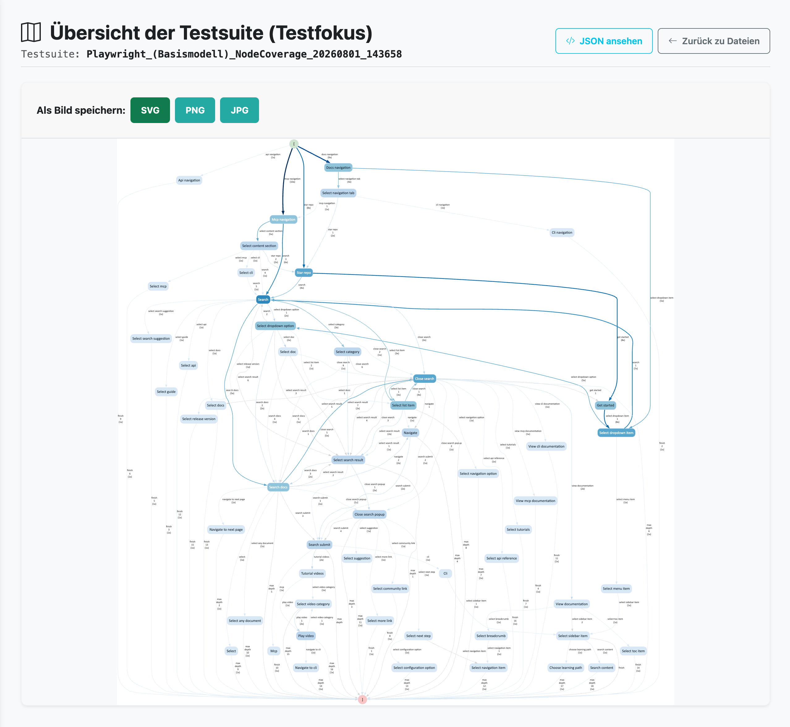
Figure 46 Step 5c: The test focus of the suite shows a 100% state coverage.

12.5 Analytical Evaluation of Frequencies

Alongside the graph, the system provides bar charts to analytically evaluate the distribution of visits. Here, it can be seen whether the automatic test generation disproportionately frequents certain states or events.

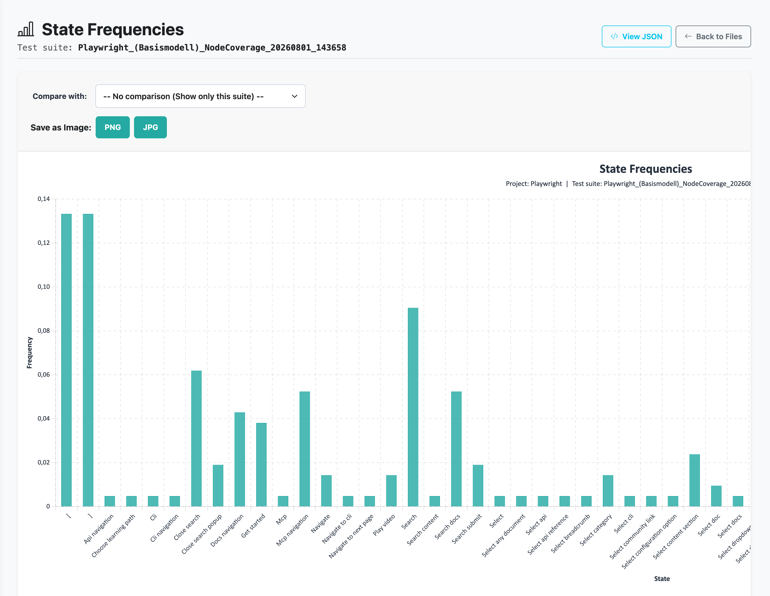
Figure 47 Step 6a: Analytical evaluation of the achieved state frequencies.

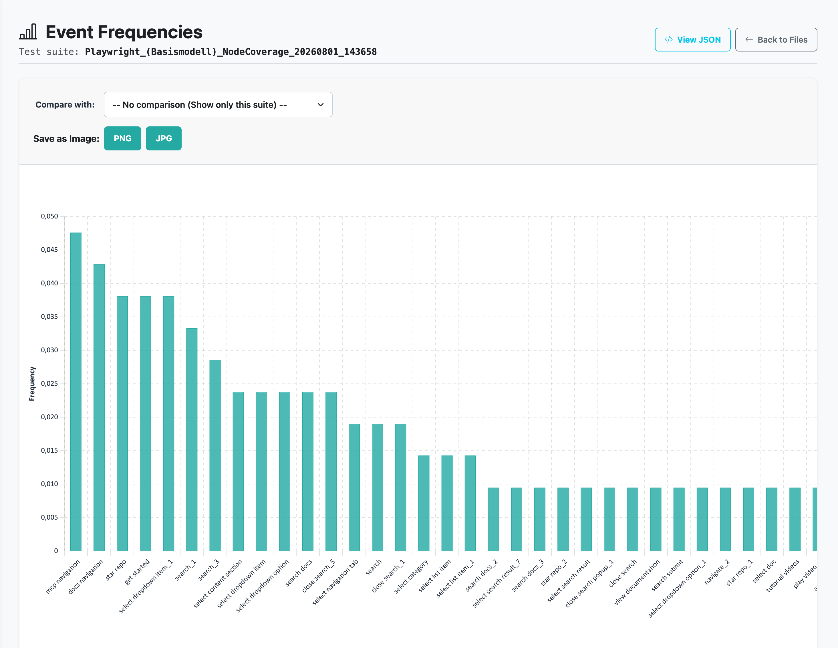
Figure 48 Step 6b: Distribution of the executed events (UI interactions).

12.6 Execution and the First “FAIL”

The validation is complete, and the suite is sent to the live website for execution via the background worker (Q-Cluster).

Since the underlying model was entirely generated by AI/heuristics, the machine-generated CSS locators in the associated SUT adapter are partially susceptible to minimal layout shifts of the website. Exactly this scenario occurs during the test run: An element is not found in time, and the Playwright agent throws a timeout. The system intercepts this and marks the test run as well as the specific event with a FAIL.

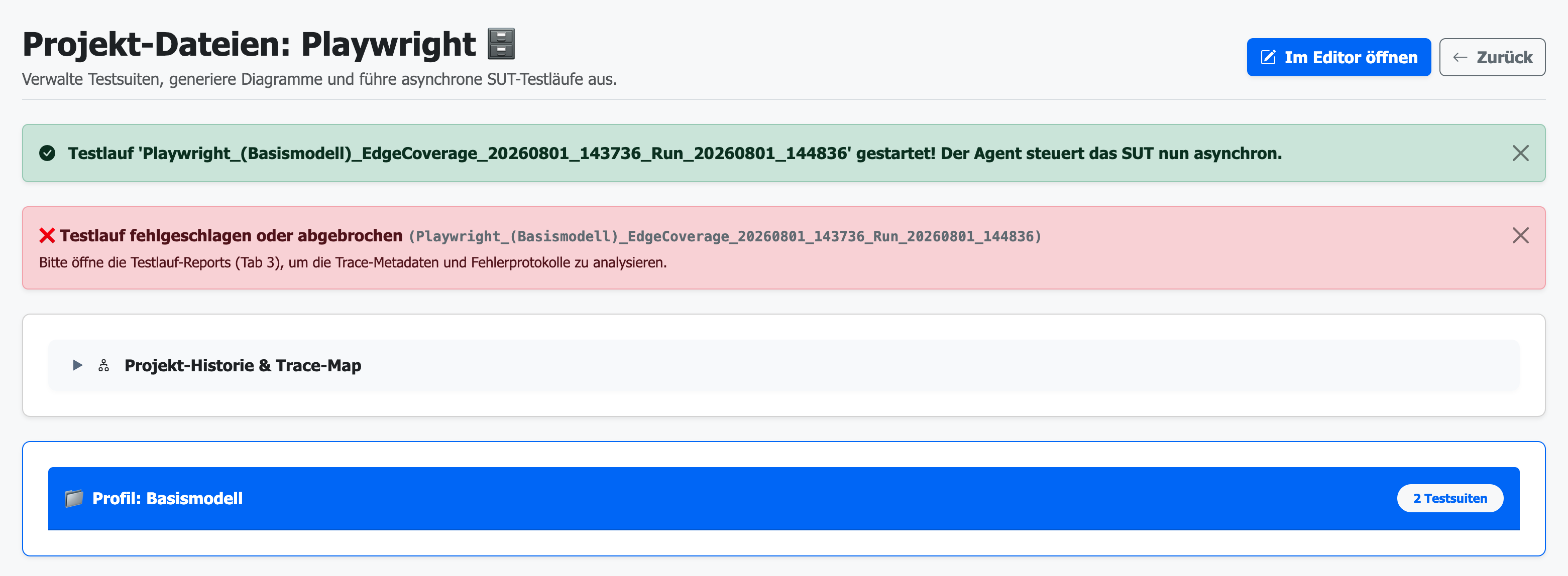
Figure 49 Step 7: The real test run aborts because an auto-discovery locator fails on the live page.

12.7 SUT Adapter Debugging and Troubleshooting

In practice, the cause of such aborts is often outdated or incorrectly generated locators (e.g., due to dynamic UI changes or inaccurate auto-discovery paths), which result in the Playwright agent being unable to interact with the System Under Test.

Step 1: Identification of the error in the dashboard

During the execution of a generated test suite, the test run aborts unexpectedly. The dashboard immediately shows in the “Test Case Breakdown” accordion where the error occurred. In the present case, test case #3 failed at the event star repo. To be able to immediately identify the cause of the error without manual reproduction, the TestPlayer automatically generates and saves the corresponding Playwright trace in a .zip archive. Via the “Trace” button, the recording of the failed run is loaded directly from the database and opened in the Playwright Trace Viewer. This visually provides the exact DOM state, network requests, action history, and all console outputs at exactly the time of the abort.

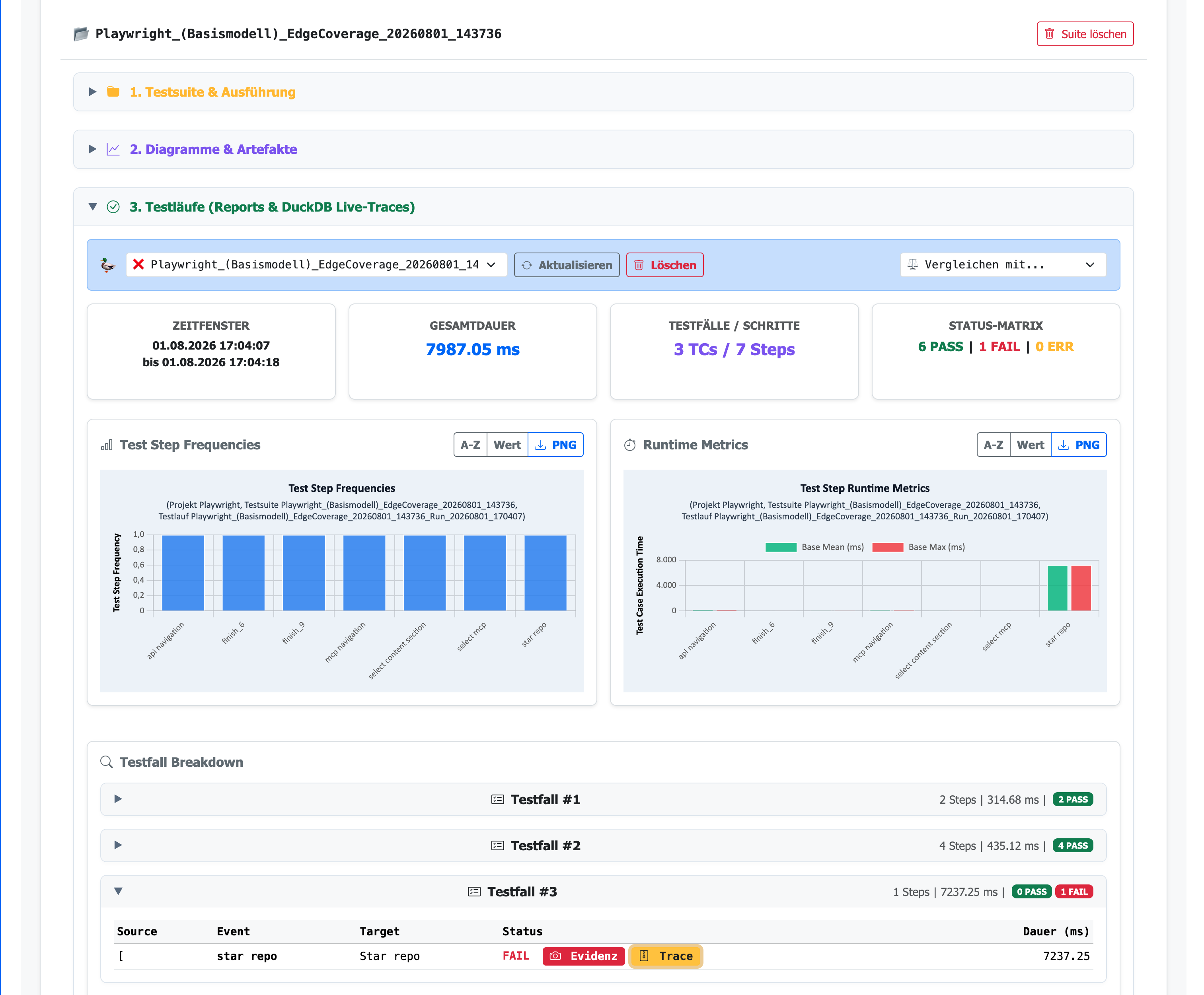
Figure 50 Step 1: Identification of the abort (FAIL) in the event “star repo” and start of the trace analysis.

Step 2: Analysis of the timeout in the Trace Viewer

The Playwright Trace Viewer automatically jumps to the end of the recording. In the “Errors” tab as well as in the source code panel below, the reason for the crash is evident: A Timeout 3000ms exceeded. The engine tried in vain for the configured 3 seconds to find the element for the event star repo in the DOM and click it.

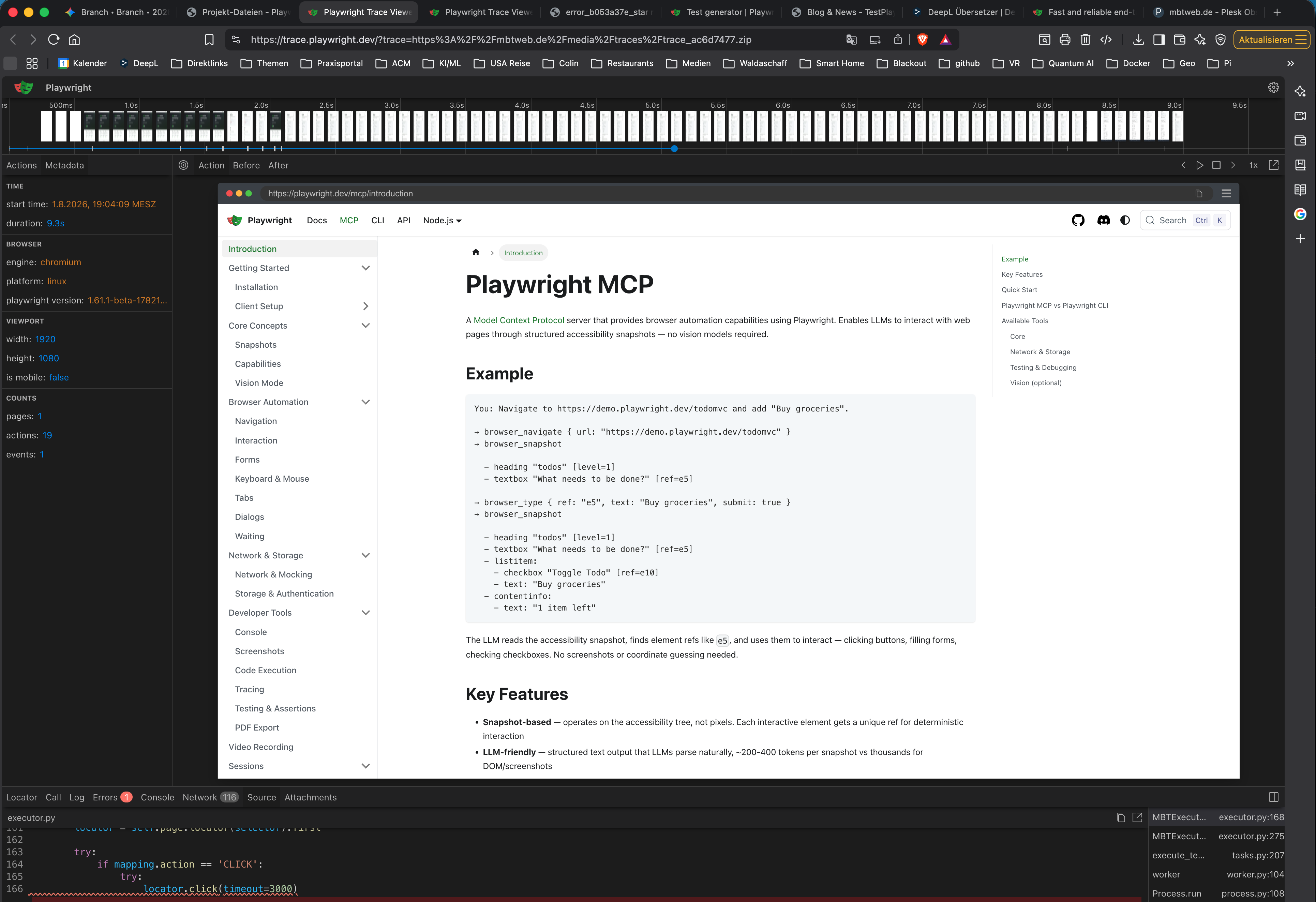
Figure 51 Step 2: The Trace Viewer reveals the exact time and cause of the timeout.

Step 3: Localization of the correct element

To fix the error, it must be found out how the target element (star repo button/link) can be addressed instead. Using the DOM inspection in the Trace Viewer (or via the developer tools of your own browser on the SUT page), a robust and unique selector is searched for. Instead of an unreliable, generated ID path (#_docusaurus_skip...), a direct CSS selector pointing to the href attribute proves to be a more stable solution here.

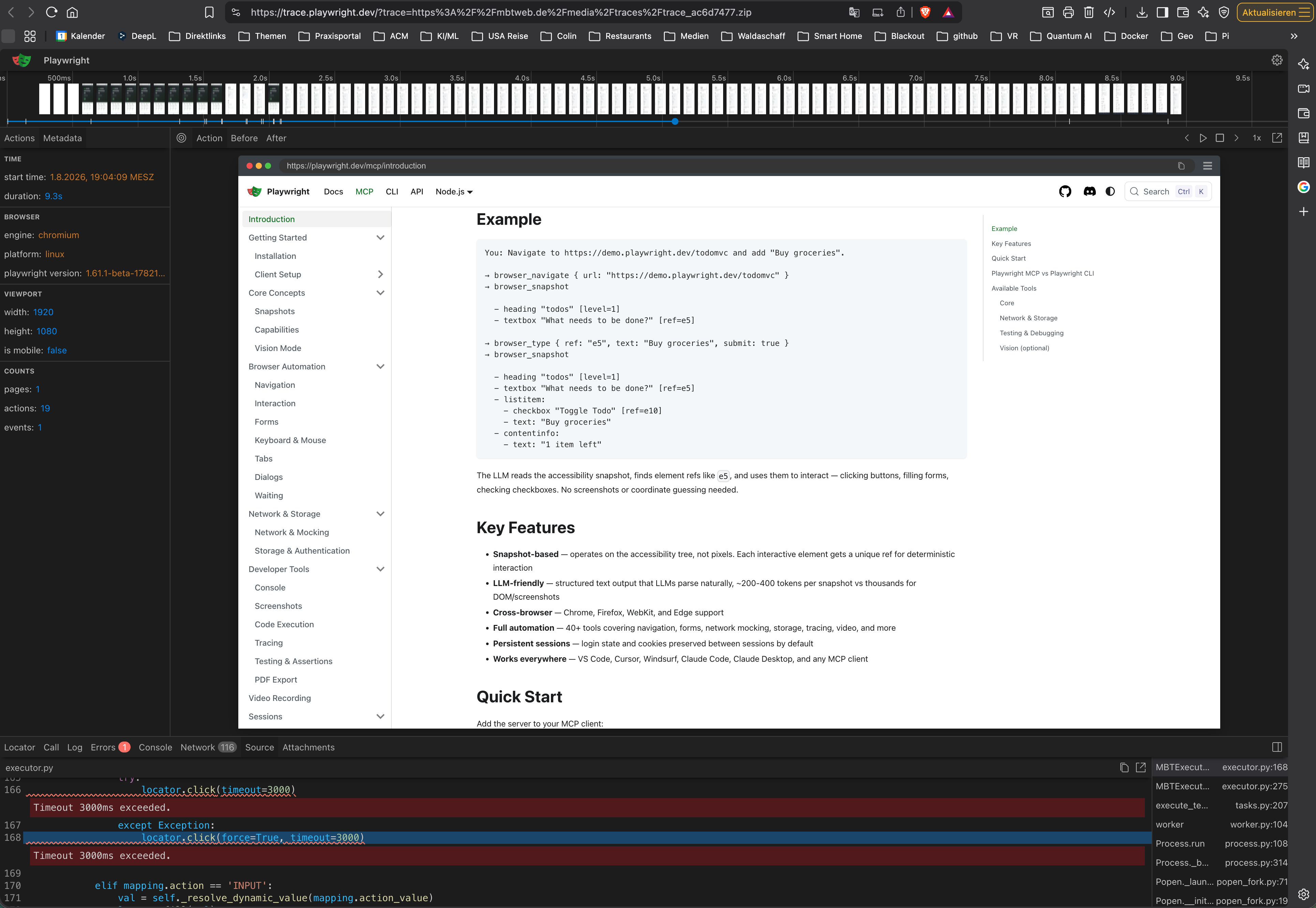
Figure 52 Step 3: Inspection of the rendered DOM to determine a robust replacement locator.

Step 4: Navigation to the SUT Adapter

Knowing the faulty selector, the user navigates via the portal menu to the SUT-Adapter Manager and opens the affected adapter (here: “Auto-Discovery (Project 15)”). The Abstract Event star repo is located in the “Event Mappings”. It is easy to see that the current Locator Type (CSS Selector) and the Value are incorrect or outdated.

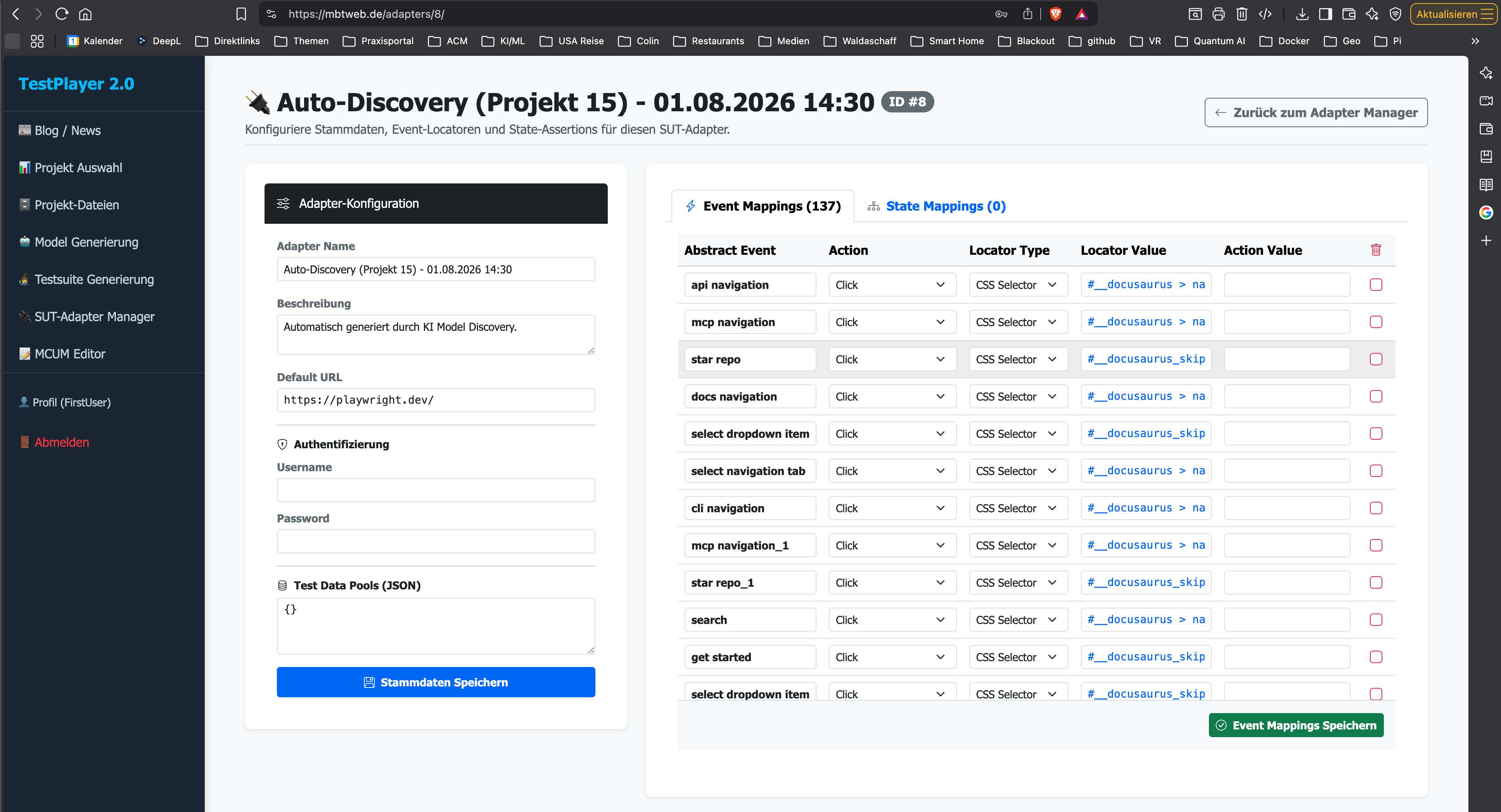
Figure 53 Step 4: Locating the faulty event mapping in the SUT Adapter Manager.

Step 5: Adjustment and saving of the mapping

The old Locator Value is replaced by the newly determined, robust selector (in this case a[href="https://g..."]). Clicking on “Save Event Mappings” writes the change live to the PostgreSQL database. The green banner confirms the successful update. The SUT adapter is now back in sync with the reality of the application.

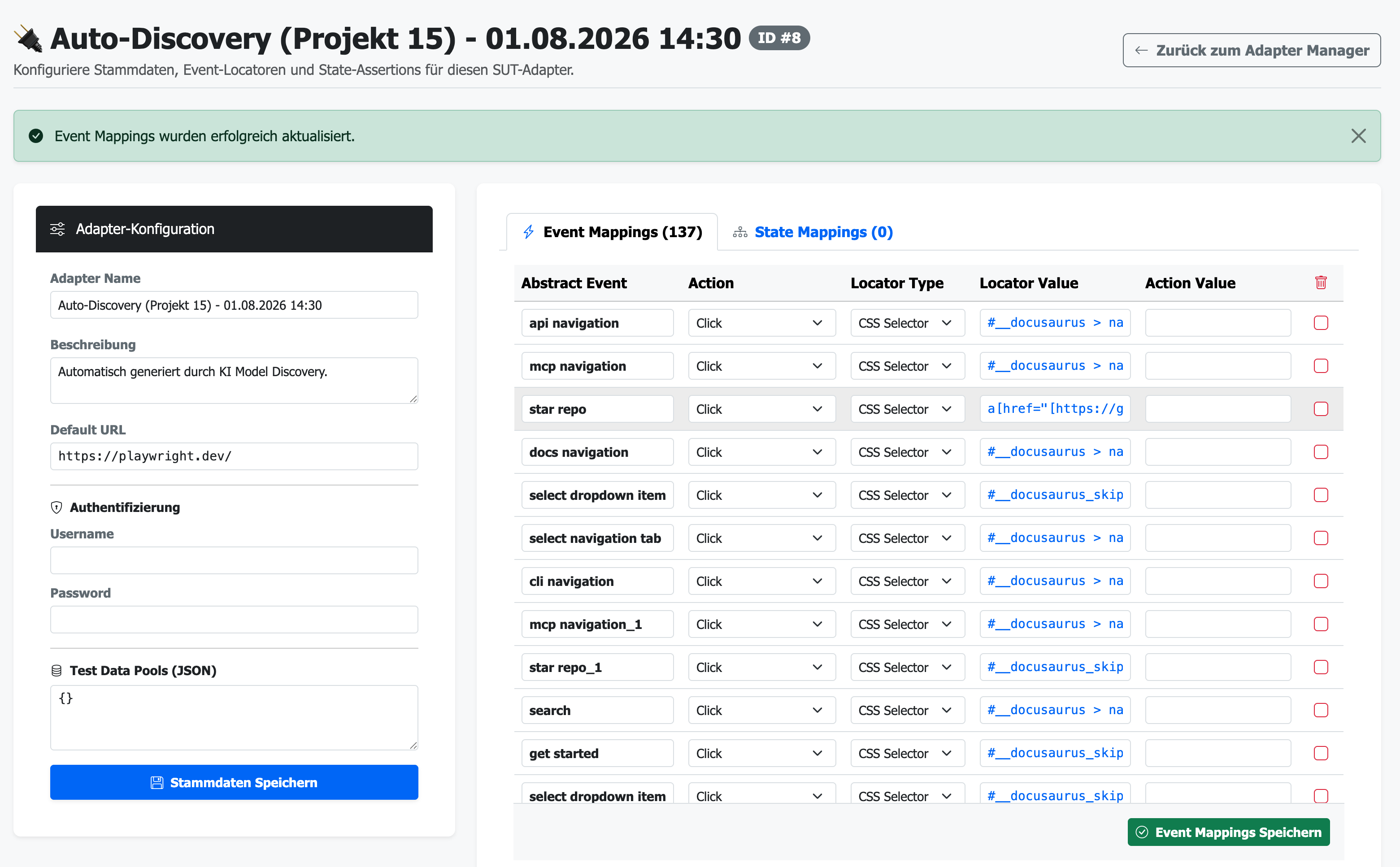
Figure 54 Step 5: In-Place update of the locator and saving in the database.

Step 6: Successful Retest

The faulty test suite can now simply be executed again without regeneration. Since the TestPlayer dynamically accesses the current mappings of the SUT adapter at every start, the correction takes effect immediately. The dashboard banner now indicates a “Successful completion of the test run”. The bottleneck was eliminated and the test coverage is guaranteed again.

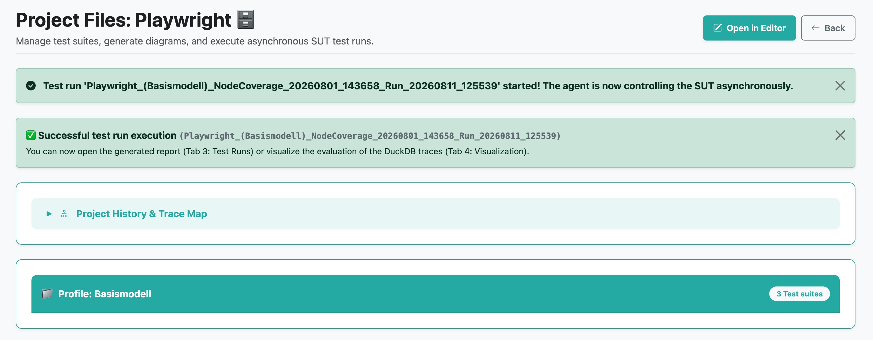
Figure 55 Step 6: The renewed test run completes successfully thanks to the corrected SUT adapter.

12.9 Performance Analysis with Playwright

TestPlayer 2.0 not only provides detailed metrics on test coverage but also deep insights into the actual execution performance of the System Under Test (SUT). The integrated debugging ecosystem utilizes the full power of the Playwright Automation Engine [4] to granularly break down bottlenecks and root causes of errors.

12.9.1 Extended Time Metrics: Time Window, Real Task Duration, and Trace Duration

The “Time Window” is extremely important for historical contextualization and the correlation of load peaks (e.g., nightly cron jobs vs. server deployments). To be able to evaluate the performance and system throughput holistically, the test run dashboard now evaluates three crucial time metrics on the upper overview cards:

• Time Window: The absolute calendar period (e.g., 01.08.2026 23:33:47 to 01.08.2026 23:33:51) in which the test run took place on the system. This chronological classification is essential to align test results and latencies with other system events (such as server deployments, load peaks, or nightly cron jobs).

• Trace Duration (ms): The pure interaction time of the Playwright Automation Engine on the DOM (e.g., 670.25 ms) for the final rendering and clicking within the virtual browser instance).

• Real Duration (Task) (s): The “wall-clock” total time (Real Execution Time) that the asynchronous Django-Q background worker requires for the complete processing of the test run task (e.g., 2.93 s). This includes starting the test matrix, the asynchronous DuckDB data preparation, and the final saving in the relational PostgreSQL model.

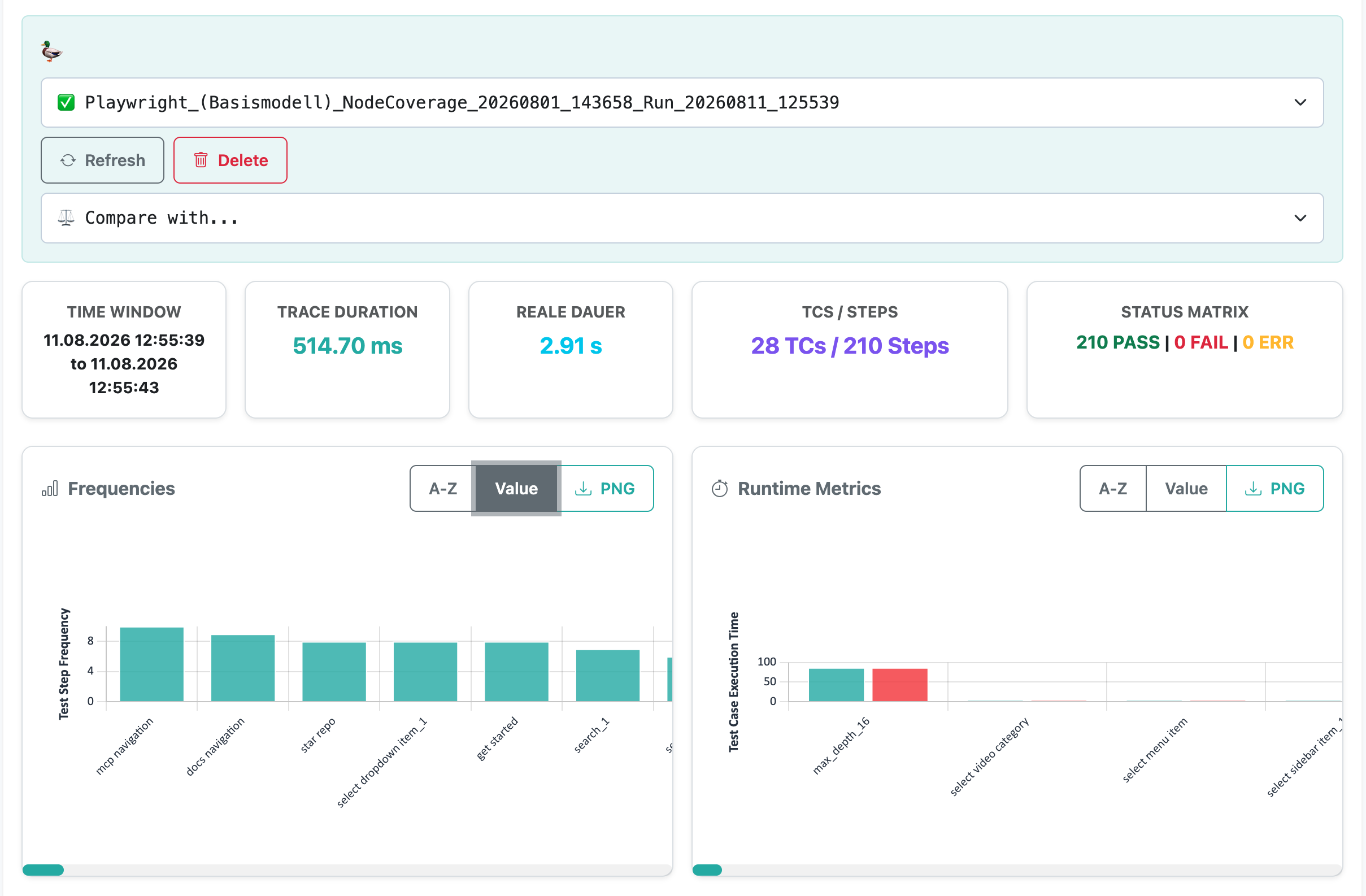
Figure 56 Distinguishing between chronological classification, the total runtime of the asynchronous task, and the Playwright trace interaction alone.

12.9.2 Analysis of Latency Outliers

The combination of performance metrics and Playwright traces enables highly precise analyses of the SUT response times.

The Scenario:

When analyzing the Execution Times of the successful test run, an apparent bottleneck was noticed in the dashboard: A specific navigation step (select navigation tab in the Docusaurus header bar) generates “outliers” averaging ~60 to 85 ms, while simple DOM clicks were processed in 1 to 40 ms.

The Investigation:

In the chronological action list (Actions tab), the specific click step could be isolated based on its locator path and the execution time of exactly 84 ms. The internal call log of Playwright revealed the exact breakdown of what these milliseconds were invested in:

• ~26 ms - Locator Resolution: The searching of the current, rendered DOM tree by the Chromium engine to identify the element based on the complex CSS selector (#__docusaurus > nav > div > div > a:nth-of-type(5)).

• ~18 ms - Actionability Checks: The mandatory waiting of the engine for the state “visible, enabled and stable”. Playwright ensures through continuous checks that the element (e.g., due to CSS animations in the header or layout shifts during loading) does not slip out from under the virtual cursor.

• ~7 ms - Viewport Calculation: The position calculation to validate whether scrolling (scrolling into view if needed) within the 1920x1080 viewport is necessary.

• ~18 ms - Physical Click Simulation: Instead of an immediate JavaScript .click(), Playwright simulates a real human at the protocol level. This requires synchronously firing mousedown, mouseup, and click events, which takes physical time.

• ~15 ms - Navigation Trigger: The registration by the browser that a page change was initiated via the <a href="..."> link.

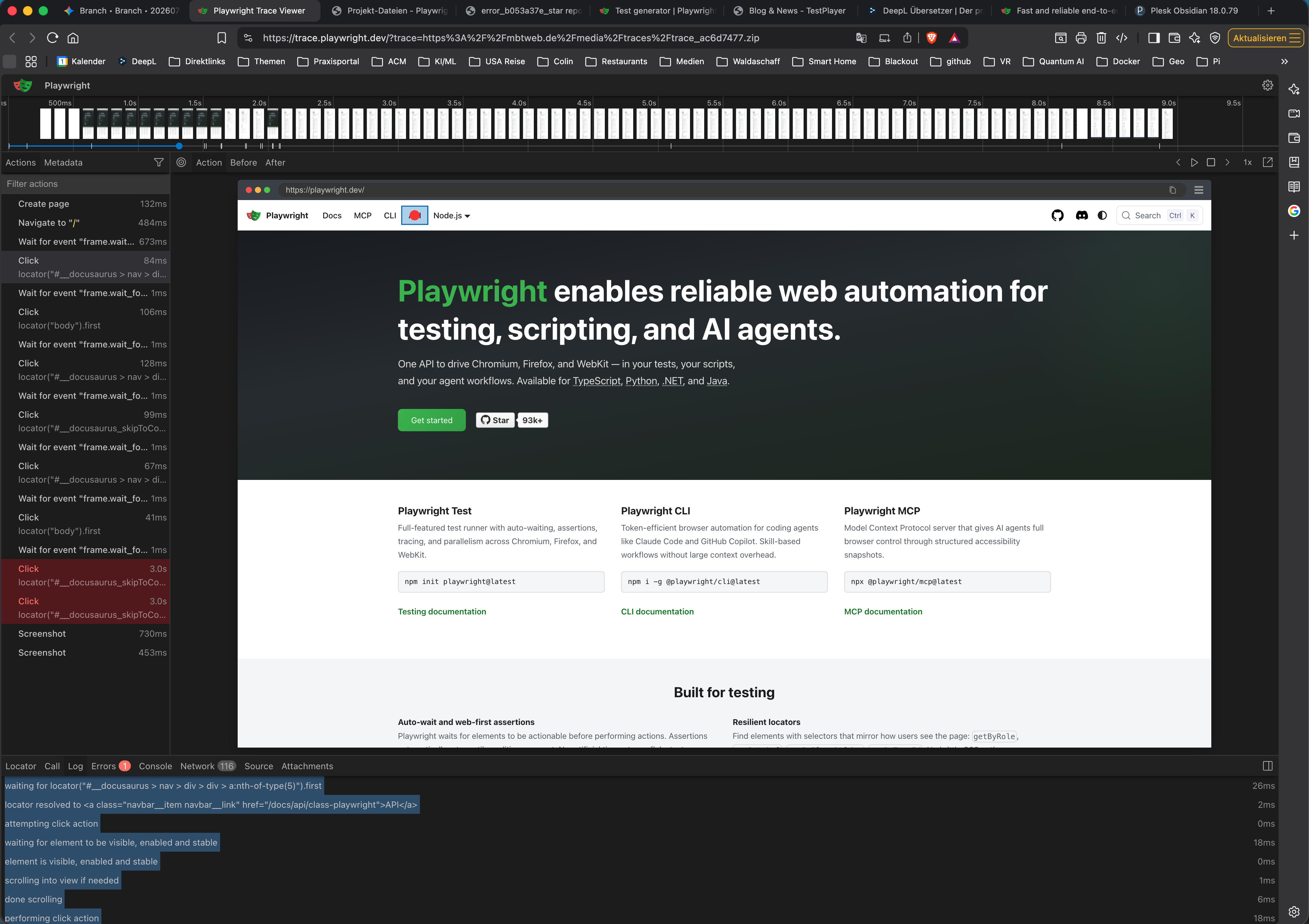
Figure 57 Isolation of the click event and breakdown of the latency in the call log of the Trace Viewer.

The Result:

What initially appeared as an “outlier” in the performance graph proved upon closer inspection to be evidence of the extreme precision and stability of the system. The measured times do not represent a bottleneck in the asynchronous processing of TestPlayer 2.0, but reflect the hard, physical limits of the rendering engine when executing realistic, validated user interactions. The observed end-to-end automation operates exactly within this time window.

13. Best Practices in Model-Based Testing (MBT)

The automated use of Model-Based Testing and Auto-Discovery generates an immense amount of system interactions in a short time. To prevent data corruption and guarantee meaningful test results, a systematic approach when testing web applications is strictly required.

13.1 SUT Isolation (The Staging Rule)

Never let automated test agents or the Auto-Discovery Engine loose on a productive live environment. The agent clicks on all reachable links, fills out forms, and could trigger real business processes (e.g., orders, email dispatches). Always set up a dedicated staging, QA, or sandbox environment for the target system and explicitly store this secure address as the default_url in the SUT adapter.

13.2 The Dedicated Bot Account

Create a special bot user in the database of the external target system (SUT) (e.g., discovery_bot@example.com).

• Secure Permissions: Assign exclusively the rights of a regular user. This realistically maps the genuine Customer Journey and prevents the agent from advancing into administrative areas.

• Configuration in TestPlayer: Enter the credentials of this bot user into the login_username and login_password fields of the respective SUT adapter. TestPlayer dynamically injects these credentials into the Automation Engine when the LOGIN_MACRO action is executed.

13.3 Test Data Hygiene and Teardown Strategies

After intensive test runs or an extensive Auto-Discovery phase, the resulting data clutter must be systematically cleaned up. A strict distinction must be made between local and remotely generated data:

• Local Cleanup (In TestPlayer): Unwanted dummy graphs, generated test suites, and recorded trace files are deleted directly via the TestPlayer UI. Clicking on “Delete suite” triggers the delete_diagram_folder route, which removes the database entries as well as orphaned physical artifacts on the server. Alternatively, dedicated backend scripts are available for mass deletions.

• Remote Cleanup (In the Target System): TestPlayer cannot automatically clean up external target systems. The SUT must be reset from within. The most efficient method here is the Cascade-Delete: Log into the backend of the target system and delete the dedicated bot user. Provided the target system has clean relational database structures, all test data generated by this user will automatically and completely cascade-deleted.

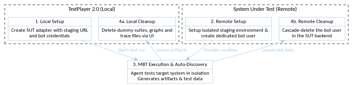
Figure 58 Systematic MBT Workflow: Strict separation of local test artifacts and remote SUT states.

Glossary

Model-Based Testing (MBT)

A software testing method in which test cases are systematically derived from an abstract behavioral model of the software to be tested.

Markov Chain Usage Model (MCUM)

A stochastic model that represents user behavior through states and transition-related probabilities.

Fundamental Matrix (N)

A matrix in the theory of absorbing Markov chains, calculated by \(N = (I - Q)^{-1}\), which indicates how often a transient state is visited on average before the final state is reached.

Ground Truth

The original visual and topological layout of the DOT model, which is preserved exactly even with dynamic color and edge adjustments by the engine.

Set Cover Problem

A mathematical optimization problem. Used in TestPlayer to filter redundant test cases from a generated suite (greedy algorithm with post-pruning).

Bibliography

[1] Dulz, W. (2026). Smart Testing 2.0: AI-driven practice and Markov Chain models. Independent Publishing.

[2] Graphviz Documentation. (2024). DOT Language and Layout Engines. Graphviz.org.

[3] D3.js & Chart.js. (2024). Interactive Data Visualization for the Web.

[4] Playwright Automation Engine. (2026). Playwright - Web automation for testing, scripting, and AI agents. Microsoft.

---

TestPlayer 2.0 – Administration Manual

The administration backend of TestPlayer 2.0 is based on the Django administration interface. It offers the platform administrator an interface for the deep configuration of the system environment, user management, and the monitoring of asynchronous execution processes.

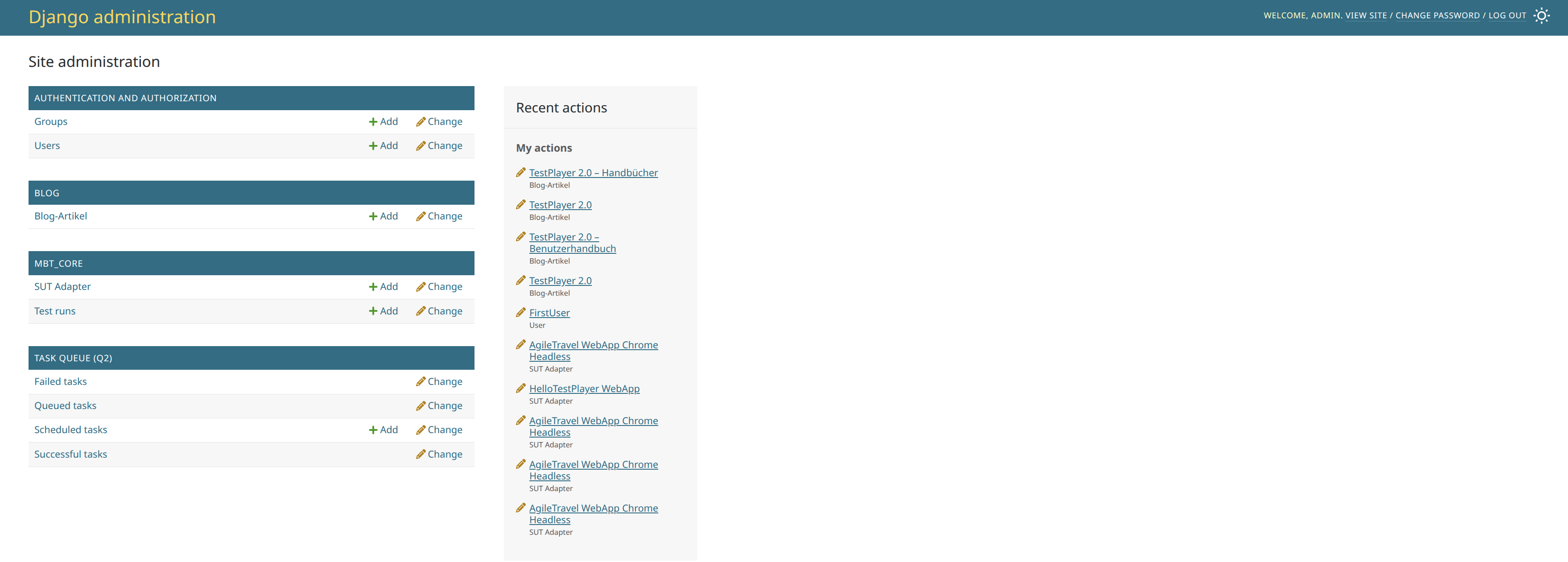
Figure 59 Administration backend of TestPlayer 2.0.

1. Authentication and Authorization

The access control of the platform is managed in this area.

• Groups: Creation and management of rights groups. Logical permission bundles can be tied here in order to assign specific system rights collectively to different user classes (e.g., standard testers vs. administrators).

• Users: Management of all registered system users. Allows resetting passwords, defining the activity status, as well as assigning users to the previously defined groups.

2. Blog

The portal for direct communication with end-users.

• Blog Articles: The content management module for creating, editing, and publishing news posts and release notes. The entries maintained here appear directly in the News & Updates section of the TestPlayer dashboard.

3. MBT_Core (Test Control)

The command center for connecting external target systems and the metadata management of executions.

3.1 SUT Adapter Management (Web-UI vs. Django-Admin)

SUT adapters control the translation between the model and execution. The primary contact point for functional testers and test automators is the SUT-Adapter Manager Web-UI (see User Manual, Chapter 6).

In the Django admin backend (MBT_Core -> SUT Adapter), administrators can additionally perform system-wide batch operations or inspect the raw data of adapters.

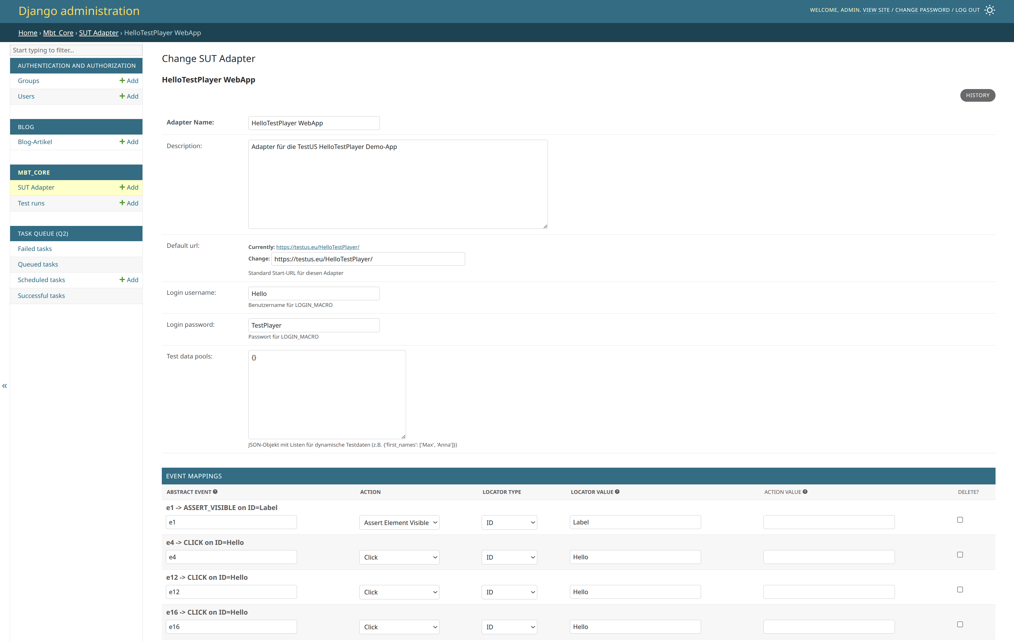
Figure 60 Django Admin view of the SUT adapter master and inline data.

3.2 SUT Adapter Lifecycle (Export / Transform / Import)

For a seamless integration of automatically discovered UI models (Auto-Discovery) and manually enriched reference models, a dedicated workflow exists via the command line interface (CLI). Data management occurs via JSON files in the directory mbt_core/management/data/sut_adapter/.

• Export (export_adapter): Exports an existing SUT adapter from the database into a JSON file to save it as a baseline or backup.

• Command: python manage.py export_adapter "<Adapter Name>"

• Transformation (transform_adapter): The core of the Auto-Discovery workflow. This script utilizes Heuristic Matching (Fuzzy Matching) to marry structural locators (e.g., nested CSS paths) from an Auto-Discovery adapter with semantic locators (e.g., clean XPATHs) from a reference adapter.

• Command: python manage.py transform_adapter "<Auto-Discovery Adapter>" "<Reference Adapter>"

• Import (import_adapter): Loads the successfully transformed SUT adapter from the JSON file back into the database so that it is available for test execution.

• Command: python manage.py import_adapter "<Transformed Adapter Name>"

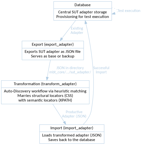
Figure 61 The workflow: From the auto-discovery model via heuristic matching to the productive adapter.

3.3 Test Data Pools & Variable Mapping

To supply generated test cases with dynamic test data (without hardcoding the test logic), TestPlayer 2.0 supports Test Data Pools.

• Variable Syntax: In the event mappings of an SUT adapter, placeholders in the form of {{variable}} can be defined in the action_value field (e.g., {{travelDay}} or {{toPort}}). The JSON test data pools resolve these variables at runtime.

• Heuristic Transfer: During transformation (via transform_adapter), the heuristic recognizes domain synonyms (e.g., destination = toPort) and automatically transfers not only the preferred locators but also the variable syntax ({{variable}}) into the new SUT adapter.

3.4 Test Runs

Overview of all asynchronously started test runs. Allows the administrator direct insight into the metadata of a run and the manual deletion of erroneous or orphaned entries to keep the database clean.

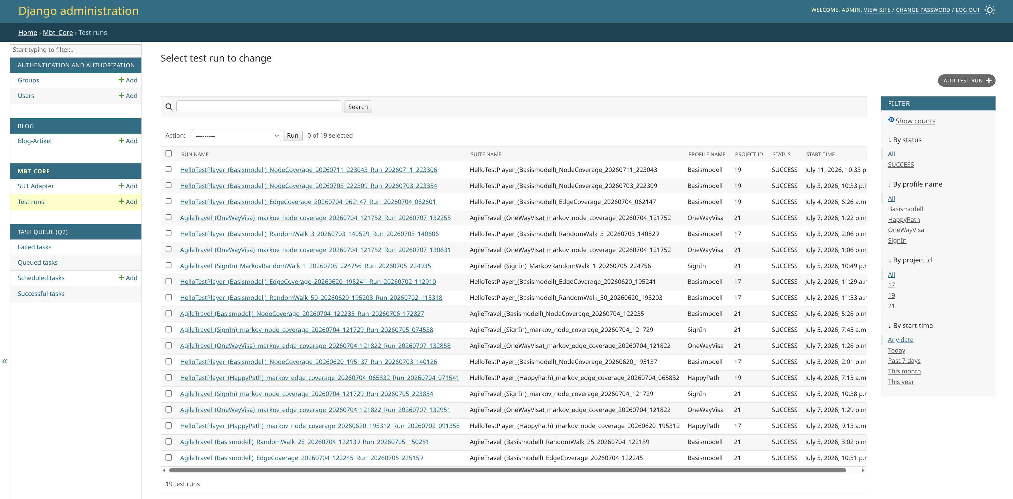
Figure 62 Overview of all asynchronously started test runs.

4. Task Queue (Q2)

This sector provides full control and visibility into the Django-Q cluster, which is responsible for the asynchronous Playwright execution (MBTExecutor) in the background.

• Failed tasks: An essential view for debugging. Tasks (such as test runs) that were aborted due to errors (e.g., Playwright timeouts, network problems) end up here, including the complete stack traces.

• Queued tasks: Test runs that are currently waiting for a free background worker and are not yet executing.

• Scheduled tasks: Management of time-controlled, recurring tasks (cron jobs).

• Successful tasks: The historical log of all successfully completed background operations.

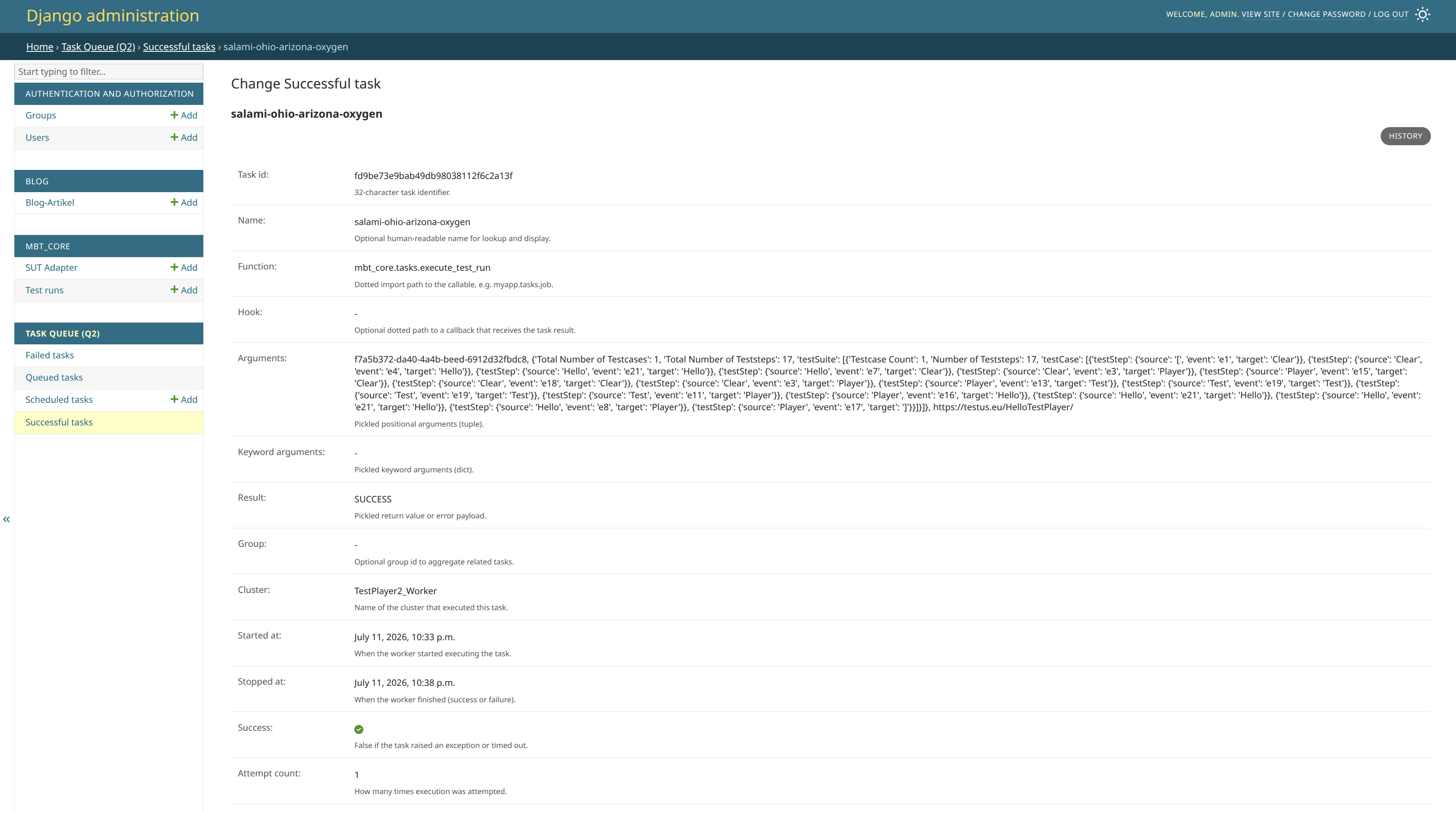
Figure 63 Log of all successfully completed background Q2 operations.